Standardized Measurement Error now available in BrainVision Analyzer and MNE-Python

A few years ago, we developed a universal metric of data quality for averaged ERPs called the standardized measurement error (click here for more information). It has been available in ERPLAB for several years, and I’m happy to announce that it is now available in BrainVision Analyzer 2.3.1 and in MNE-Python.

For BrainVision Analyzer, it is available as a Solution. At this point, you need to request it from Brain Products. Click here and scroll down to the last part of the page for more information.

For MNE-Python, it is accessed with the mne.stats.erp.compute_sme() function. Click here for details.

If you want to see some examples of how this metric can be used, check out these recent papers:

  • Zhang, G., Garrett, D. R., & Luck, S. J. (2024a). Optimal filters for ERP research I: A general approach for selecting filter settings. Psychophysiology, 61, e14531. http://doi.org/10.1111/psyp.14531 [preprint]

  • Zhang, G., Garrett, D. R., & Luck, S. J. (2024b). Optimal filters for ERP research II: Recommended settings for seven common ERP components. Psychophysiology, 61, e14530. https://doi.org/10.1111/psyp.14530 [preprint]

  • Zhang, G., Garrett, D. R., Simmons, A. M., Kiat, J. E., & Luck, S. J. (2024). Evaluating the effectiveness of artifact correction and rejection in event-related potential research. Psychophysiology, 61, e14511. https://doi.org/10.1111/psyp.14511 [preprint]

  • Zhang, G., & Luck, S. J. (2023). Variations in ERP data quality across paradigms, participants, and scoring procedures. Psychophysiology, 60, e14264. http://doi.org/10.1111/psyp.14264 [preprint]

New Paper: Using Multivariate Pattern Analysis to Increase Effect Sizes for ERP Amplitude Comparisons

Carrasco, C. D., Bahle, B., Simmons, A. M., & Luck, S. J. (2024). Using multivariate pattern analysis to increase effect sizes for event-related potential analyses. Psychophysiology, 61, e14570. https://doi.org/10.1111/psyp.14570 [preprint]

Multivariate pattern analysis (MVPA) can be used to “decode” subtle information from ERP signals, such as which of several faces a participant is perceiving or the orientation that someone is holding in working memory (see this previous blog post). This approach is so powerful that we started wondering whether it might also give us greater statistical power in more typical experiments where the goal is to determine whether an ERP component differs in amplitude across experimental conditions. For example, might we more easily be able to tell if N400 amplitude is different between two different classes of words by using decoding? If so, that might make it possible to detect effects that would otherwise be too small to be significant.

To address this question, we compared decoding with the conventional ERP analysis approach with using the 6 experimental paradigms in the ERP CORE. In the conventional ERP analysis, we measured the mean amplitude during the standard measurement window from each participant in the two conditions of the paradigm (e.g., faces versus cars for N170, deviants versus standards for MMN). We quantified the magnitude of the difference between conditions using Cohen’s dz (the variant of Cohen’s d corresponding to a paired t test). For example, the effect size in the conventional ERP comparison of faces versus cars in the N170 paradigm was approximately 1.7 (see the figure).

We also applied decoding to each paradigm. For example, in the N170 paradigm, we trained a support vector machine (SVM) to distinguish between ERPs elicited by faces and ERPs elicited by cars. This was done separately for each subject, and we converted the decoding accuracy into Cohen’s dz so that it could be compared with the dz from the conventional ERP analysis. As you can see from the bar labeled SVM in the figure above, the effect size for the SVM-based decoding analysis was almost twice as large as the effect size for the conventional ERP analysis. That’s a huge difference!

We found a similar benefit for SVM-based decoding over conventional ERP analyses in 7 of the 10 cases we tested (see the figure below). In the other 3 cases, the ERP and SVM effects were approximately equivalent. So, there doesn’t seem to be a downside to using decoding, at least in terms of effect size. But there can be a big benefit.

Because decoding has many possible benefits, we’ve added it into ERPLAB Toolbox. It’s super easy to use, and we’ve created detailed documentation and a video to explain how it works at a conceptual level and to show you how to use it.

We encourage you to apply it to your own data. It may give you the power to detect effects that are too small to be detected with conventional ERP analyses.

New Papers: Optimal Filter Settings for ERP Research

Zhang, G., Garrett, D. R., & Luck, S. J. (in press). Optimal filters for ERP research I: A general approach for selecting filter settings. Psychophysiology. https://doi.org/10.1111/psyp.14531 [preprint]

Zhang, G., Garrett, D. R., & Luck, S. J. (in press). Optimal filters for ERP research II: Recommended settings for seven common ERP components. Psychophysiology. https://doi.org/10.1111/psyp.14530 [preprint]

What filter settings should you apply to your ERP data? If your filters are too weak to attenuate the noise in your data, your effects may not be statistically significant. If your filters are too strong, they may create artifactual peaks that lead you to draw bogus conclusions.

For years, I have been recommending a bandpass of 0.1–30 Hz for most cognitive and affective research in neurotypical young adults. In this kind of research, I have found that filtering from 0.1–30 Hz usually does a good job of minimizing noise while creating minimal waveform distortion.

However, this recommendation was based on a combination of informal observations from many experimental paradigms and a careful examination of a couple paradigms, so it was a bit hand-wavy. In addition, the optimal filter settings will depend on the waveshape of the ERP effects and the nature of the noise in a given study, so I couldn’t make any specific recommendations about other experimental paradigms and participant populations. Moreover, different filter settings may be optimal for different scoring methods (e.g., mean amplitude vs. peak amplitude vs. peak latency).

Guanghui Zhang, David Garrett, and I spent the last year focusing on this issue. First we developed a general method that can be used to determine the optimal filter settings for a given dataset and scoring method (see this paper). Then we applied this method to the ERP CORE data to determine the optimal filter settings for the N170, MMN, P3b, N400, N2pc, LRP, and ERN components in neurotypical young adults (see this paper and the table above).

If you are doing research with these components (or similar components) in neurotypical young adults, you can simply use the filter settings that we identified. If you are using a very different paradigm or testing a very different subject population, you can apply our method to your own data to find the optimal settings. We added some new tools to ERPLAB Toolbox to make this easier.

One thing that we discovered was that our old recommendation of 0.1–30 Hz does a good job of avoiding filter artifacts but is overly conservative for some components. For example, we can raise the low end to 0.5 Hz when measuring N2pc and MMN amplitudes, which gets rid of more noise without producing problematic waveform distortions. And we can go all the way up to 0.9 Hz for the N170 component. However, later/slower components like P3b and N400 require lower cutoffs (no higher than 0.2 Hz).

You might be wondering how we defined the “optimal” filter settings. At one level, the answer is simple: The optimal filter is the one that maximizes the signal-to-noise ratio without producing too much waveform distortion. The complexities arise in quantifying the signal-to-noise ratio, quantifying the waveform distortion, and deciding how much waveform distortion is “too much”. We believe we have found reasonably straightforward and practical solutions to these problems, which you can read about in the published papers.

ERP Decoding for Everyone: Software and Webinar

You can access the recording here.
You can access the final PDF of the slides
here.
You can access the data
here.

fMRI research has used decoding methods for over 20 years. These methods make it possible to decode what an individual is perceiving or holding in working memory on the basis of the pattern of BOLD activity across voxels. Remarkably, these methods can also be applied to ERP data, using the pattern of voltage across electrode sites rather than the pattern of activity across voxels to decode the information being represented by the brain (see this previous blog post). For example, ERPs can be used to decode the identity of a face that is being perceived, the emotional valence of a scene, the identity and semantic category of a word, and the features of an object that is being maintained in working memory. Moreover, decoding methods can be more sensitive than traditional methods for detecting conventional ERP effects (e.g., whether a word is semantically related or unrelated to a previous word in an N400 paradigm).

So far, these methods have mainly been used by a small set of experts. We aim to change that with the upcoming Version 10 of ERPLAB Toolbox. This version of ERPLAB will contain an ERP decoding tool that makes it trivially easy for anyone who knows how to do conventional ERP processing to take advantage of the power of decoding. It should be available in mid-July at our GitHub site. You can join the ERPLAB email list to receive an announcement when this version is released. Please do not contact us with questions until it has been released and you have tried using it.

On July 25, 2023, we will hold a 2-hour Zoom webinar to explain how decoding works at a conceptual level and show how to implement in ERPLAB Toolbox. The webinar will begin at 9:00 AM Pacific Time (California), 12:00 PM Eastern Time (New York), 5:00 PM British Summer Time (London), 6:00 PM Central European Summer Time (Berlin).

The webinar is co-sponsored by the ERP Boot Camp and the Society for Psychophysiological Research. It is completely free, but you must register in advance at https://ucdavis.zoom.us/meeting/register/tJUrc-CtpzorEtBSmZXJINOlLJB9ZR0evpr4. Once you register, you will receive an email with your own individual Zoom link.

We will make a recording available a few days after the webinar on the ERPinfo.org web site.

Please direct any questions about the webinar to erpbootcamp@gmail.com.

New Book: Applied ERP Data Analysis

I’m excited to announce my new book, Applied ERP Data Analysis. It’s available online FOR FREE on the LibreTexts open source textbook platform. You can cite it as: Luck, S. J. (2022). Applied Event-Related Potential Data Analysis. LibreTexts. https://doi.org/10.18115/D5QG92

The book is designed to be read online, but LibreTexts has a tool for creating a PDF. You can then print the PDF if you prefer to read on paper.

I’ve aimed the book at beginning and intermediate ERP researchers. I assume that you already know the basic concepts behind ERPs, which you can learn from my free online Intro to ERPs course (which takes 3-4 hours to complete).

Whereas my previous book focuses on conceptual issues, the new book focuses on how to implement these concepts with real data. Most of the book consists of exercises in which you process data from the ERP CORE, a set of six ERP paradigms that yield seven different components (P3b, N400, MMN, N2pc, N170, ERN, LRP). Learn by doing!

With real data, you must deal with all kinds of weird problems and make many decisions. The book will teach you principled approaches to solving these problems and making optimal decisions.

Side note: my approach in this book was inspired by Mike X Cohen’s excellent book, Analyzing Neural Time Series Data: Theory and Practice.

You will analyze the data using EEGLAB and ERPLAB, which are free open source Matlab toolboxes. Make sure to download version 9 of ERPLAB. (You may need to buy Matlab, but many institutions provide free or discounted licenses for students.) Although you will learn a lot about these specific software packages, the exercises and accompanying text are designed to teach broader concepts that will translate to any software package (and any ERP paradigm). The logic is much more important than the software!

One key element of the approach, however, is currently ERPLAB-specific. Specifically, the book frequently asks whether a given choice increases or decreases the data quality of the averaged ERPs, as quantified with the Standardized Measurement Error (SME). If this approach makes sense to you, but you prefer a different analysis package, you should encourage the developers of that package to implement SME. All our code is open source, so translating it to a different package should be straightforward. If enough people ask, they will listen!

The book also contains a chapter on scripting, plus tons of example scripts. You don’t have to write scripts for the other chapters. But learning some simple scripting will make you more productive and increase the quality, innovation, and reproducibility of your research.

I made the book free and open source so that I could give something back to the ERP community, which has given me so much over the years. But I’ve discovered two downsides to making the book free. First, there was no copy editor, so there are probably tons of typos and other errors. Please shoot me an email if you find an error. (But I can’t realistically provide tech support if you have trouble with the software.) Second, there is no marketing budget, so please spread the word to friends, colleagues, students, and billionaire philanthropists.

This book was also designed for use in undergrad and grad courses. The LibreTexts platform makes it easy for you to create a customized version of the book. You can reorder or delete sections or whole chapters. And you can add new sections or edit any of the existing text. It’s published with a CC-BY license, so you can do anything you want with it as long as you provide an attribution to the original source. And if you don’t like some of the recommendations I make in the book, you can just change it to say whatever you like! For example, you can add a chapter titled “Why Steve Luck is wrong about filtering.”

If you are a PI: the combination of the online course, this book, and the resources provided by PURSUE give you a great way to get new students started in the lab. I’m hoping this makes it easier for faculty to get more undergrads involved in ERP research. 

Representational Similarity Analysis- A great method for linking ERPs to computational models, fMRI data, and more

Representational similarity analysis (RSA) is a powerful multivariate pattern analysis method that is widely used in fMRI, and my lab has recently published two papers applying RSA to ERPs. We’re not the first researchers to apply RSA to ERP or MEG data (see, e.g., Cichy & Pantazis, 2017; Greene & Hansen, 2018). However, RSA is a relatively new approach with amazing potential, and I hope this blog inspires more people to apply RSA to ERP data. You can also watch a 7-minute video overview of RSA on YouTube. Here are the new papers:

  • Kiat, J.E., Hayes, T.R., Henderson, J.M., Luck, S.J. (in press). Rapid extraction of the spatial distribution of physical saliency and semantic informativeness from natural scenes in the human brain. The Journal of Neuroscience. https://doi.org/10.1523/JNEUROSCI.0602-21.2021 [preprint] [code and data]

  • He, T., Kiat, J. E., Boudewyn, M. A., Segae, K., & Luck, S. J. (in press). Neural Correlates of Word Representation Vectors in Natural Language Processing Models: Evidence from Representational Similarity Analysis of Event-Related Brain Potentials. Psychophysiology. https://doi.org/10.1111/psyp.13976 [preprint] [code and data]

Examples

Before describing how RSA works, I want to whet your appetite by showing some of our recent results. Figure 1A shows results from a study that examined the relationship between scalp ERP data and a computational model that predicts the saliency of each location in a natural scene. 50 different scenes were used in the experiment, and the waveform in Figure 1A shows the representational link between the ERP data and the computational model at each moment in time. You can see that the link onsets rapidly and peaks before 100 ms, which makes sense given that the model is designed to reflect early visual cortex. Interestingly, the link persists well past 300 ms. Our study also examined meaning maps, which quantify the amount of meaningful information at each point in a scene. We found that the link between the ERPs and the meaning maps began only slightly after the link with the saliency model. You can read more about this study here.

FIGURE 1

Figure 1B shows some of the data from our new study of natural language processing, in which subjects simply listened to stories while the EEG was recorded. The waveform shows the representational link between scalp ERP data and a natural language processing model for a set of 100 different words. You can see that the link starts well before 200 ms and lasts for several hundred milliseconds. The study also examined a different computational model, and it contains many additional interesting analyses.

In these examples, RSA allows us to see how brain activity elicited by complex, natural stimuli can be related to computational models, using brain activity measured with the high temporal resolution and low cost of scalp ERP data. This technique is having a huge impact on the kinds of questions my lab is now asking. Specifically :

  • RSA is helping us move from simple, artificial laboratory stimuli to stimuli that more closely match the real world.

  • RSA is helping us move from qualitative differences between experimental conditions to quantitative links to computational models.

  • RSA is helping us link ERPs with the precise neuroanatomy of fMRI and with rich behavioral datasets (e.g., eye tracking).

Figure 1 shows only a small slice of the results from our new studies, but I hope they give you the idea of the kinds of things that are possible with RSA. We’ve also made the code and data available for both the language study (https://osf.io/zft6e/) and the visual attention study (https://osf.io/zg7ue/). Some coding is skill is necessary to implement RSA, but it’s easier than you might think (especially when you use our code and code provided by other labs as a starting point).

Now let’s take a look at how RSA works in general and how it is applied to ERP data.

The Essence of Representational Similarity Analysis (RSA)

RSA is a general-purpose method for assessing links among different kinds of neural measures, computational models, and behavior. Each of these sources of data has a different format, which makes them difficult to compare directly. As illustrated in Figure 2, ERP datasets contain a voltage value at each of several scalp electrode sites at each of several time points; a computational model might contain an activation value for each of several processing units; a behavioral dataset might consist of a set of eye movement locations; and an fMRI dataset might consist of a set of BOLD beta values in each voxel within a given brain area. How can we link these different types of data to each other? The mapping might be complex and nonlinear, and there might be thousands of individual variables within a dataset, which would limit the applicability of traditional approaches to examining correlations between datasets.

RSA takes a very different approach. Instead of directly examining correlations between datasets, RSA converts each data source into a more abstract but directly comparable format called a representational similarity matrix (RSM). To obtain an RSM, you take a large set of stimuli and use these stimuli as the inputs to multiple different data-generating systems. For example, the studies shown in Figure 1 involved taking a set of 50 visual scenes or 100 spoken words and presenting them as the input to a set of human subjects in an ERP experiment and as the input to a computational model.

As illustrated in Figure 2A, each of the N stimuli gives you a set of ERP waveforms. For each pair of the N stimuli, you can quantify the similarity of the ERPs (e.g., the correlation between the scalp distributions at given time point), leading to an N x N representational similarity matrix.

FIGURE 2

The same N stimuli would also be used as the inputs to the computational model. For each pair of stimuli, you can quantify the similarity of model’s response to the two stimuli (e.g., the correlation between the pattern of activation produced by the two stimuli). This gives you an N x N representational similarity matrix for the model.

Now we’ve transformed both the ERP data and the model results into N x N representational similarity matrices. The ERP data and the model originally had completely different units of measurement and data structures that were difficult to relate to each other, but now we have the same data format for both the ERPs and the model. This makes it simple to ask how well the similarity matrix for the ERP data matches the similarity matrix for the model. Specifically, we can just calculate the correlation between the two matrices (typically using a rank order approach so that we only assume a monotonic relationship, not a linear relationship).

Some Details

The data shown in Figure 1 used the Pearson r correlation coefficient to quantify the similarity between ERP scalp distributions. We have found that this is a good metric of similarity for ERPs, but other metrics can sometimes be advantagous. Note that many researchers prefer to quantify dissimilarity (distance) rather than similarity, but the principle is the same.

Each representational similarity matrix (RSM) captures the representational geometry of the system that produced the data (e.g., the human brain or the computational model). The lower and upper triangles of the RSM as described in this approach are mirror images of each other and are redundant. Similarly, cells along the diagonal index the similarity of each item to itself and are not considered in cross-RSM comparisons. We therefore use only the lower triangles of the RSMs. As illustrated in Figure 2a, the representational similarity between the ERP data and the computational model is simply the (rank order) correlation between the values in these two lower triangles.

When RSA is used with ERP data, representational similarity is typically calculated separately for each time point. That is, the scalp distribution is obtained at a given time point for each of the N stimuli, and the correlation between the scalp distributions for each pair of stimuli is computed at this time point. Thus, we have an N x N RSM at each time point for the ERP data. Each of these RSMs is then correlated with the RSM from the computational model. If the model has multiple layers, this process is conducted separately for each layer.

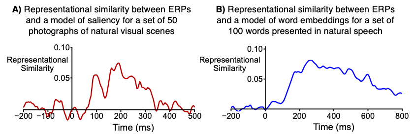
For example, the waveforms shown in Figure 1 show the (rank order) correlation between the ERP RSM at a given time point and the model RSM. That is, each time point in the waveform shows the correlation between the ERP RSM for that time point and the model RSM.

ERP scalp distributions can vary widely across people, so RSA is conducted separately for each participant. That is, we compute an ERP RSM for each participant (at each time point) and calculate the correlation between that RSM and the Model RSM. This gives us a separate ERP-Model correlation value for each participant at each time point. The waveforms shown in Figure 1 show the average of the single-participant correlations.

The correlation values in RSA studies of ERPs are typically quite low compared to the correlation values you might see in other contexts (e.g., the correlation between P3 latency and response time). For example, all of the correlation values in the waveforms shown in Figure 1 are less than 0.10. However, this is not usually a problem for the following reasons:

  • The low correlations are mainly a result of the noisiness of scalp ERP data when you compute a separate ERP for each of 50-100 stimuli, not a weak link between the brain and the model.

  • It is possible to calculate a “noise ceiling,” which represents the highest correlation between RSMs that could be expected given the noise in the data. The waveforms shown in Figure 1 reach a reasonably high value relative to the noise ceiling.

  • When the correlation between the ERP RSM and the model RSM is computed for a given participant, the number of data points contributing to the correlation is typically huge. For a 50 x 50 RSM (as in Figure 1A), there are 1225 cells in the lower triangle. 1225 values from the ERP RSM are being correlated with 1225 values from the model RSM. This leads to very robust correlation estimates.

  • Additional power is achieved from the fact that a separate correlation is computed for each participant.

  • In practice, the small correlation values obtained in ERP RSA studies are scientifically meaningful and can have substantial statistical power.

RSA is usually applied to averaged ERP waveforms, not single-trial data. For example, we used averages of 32 trials per image in the experiment shown in Figure 1A. The data shown in Figure 1B are from averages of at least 10 trials per word. Single-trial analyses are possible but are much noisier. For example, we conducted single-trial analyses of the words and found statistically significant but much weaker representational similarity.

Other Types of Data

As illustrated in Figure 2A, RSA can also be used to link ERPs to other types of data, including behavioral data and fMRI data.

The behavioral example in Figure 2A involves eye tracking. If the eyes are tracked while participants view scenes, a fixation density map can be constructed showing the likelihood that each location was fixated for each scene. An RSM for the eye-tracking data could be constructed to indicate the similarity between fixation density maps for each pair of scenes. This RSM could then be correlated with the ERP RSM at each time point. Or the fixation density RSMs could be correlated with the RSM for a computational model (as in a recent study in which we examined the relationship between infant eye movement patterns and a convolutional neural network model of the visual system; Kiat et al., 2022).

Other types of behavioral data could also be used. For example, if participants made a button-press response to each stimulus, one could use the mean response times for each stimulus to construct an RSM. The similarity value for a given cell would be the difference in mean RT between two different stimuli.

RSA can also be used to link ERP data to fMRI data, a process called data fusion (see, e.g., Mohsenzadeh et al., 2019). The data fusion process makes it possible to combine the spatial resolution of fMRI with the temporal resolution of ERPs. It can yield a millisecond-by-millisecond estimate of activity corresponding to a given brain region, and it can also yield a voxel-by-voxel map of the activity corresponding to a given time point. More details are provided in our YouTube video on RSA.

Webinar on the ERP CORE

Note: This webinar was originally scheduled for August 12, but it has been rescheduled for August 26.

We will be holding a webinar on the ERP CORE, a freely available online resource we developed for the ERP community.

The ERP CORE includes: 1) experiment control scripts for 6 optimized ERP paradigms that collectively elicit 7 ERP components (N170, MMN, N2pc, N400, P3, LRP, and ERN) in just one hour of recording time, 2) raw and processed data from 40 neurotypical young adults in each paradigm, 3) EEG/ERP data processing pipelines and analysis scripts in EEGLAB and ERPLAB Matlab Toolboxes, and 4) a broad set of ERP results and EEG/ERP data quality measures for comparison across laboratories.

Check out this blog post for more information about the ERP CORE and how you can use it.

The webinar will be presented by Emily Kappenman, and it will be held on Wednesday, August 26 at 9:00 AM Pacific Daylight Time (GMT-7). We expect that it will last 60-90 minutes.

During the webinar, we will (a) provide an overview of the ERP CORE paradigms; (b) introduce the data set, analysis files, and Matlab scripts provided in the resource; and (c) describe some ways that you might use the ERP CORE in your research.

Advance registration is required and will be limited to the first 950 registrants. You can register at https://ucdavis.zoom.us/webinar/register/WN_BlozaZr-QeW6htlBqQXtpQ.

When you register, you will immediately receive an email with an individualized Zoom link. If you do not see the email, check your spam folder. If you still don’t see it, you may have entered your email address incorrectly.

If you can’t attend, we will make a recording available for 1 week after the webinar. The link to the recording will be provided at https://erpinfo.org/virtual-boot-camp within 24 hours of the end of the webinar. You do NOT need to register to watch the recording.

Questions can be directed to erpbootcamp@gmail.com.

Webinar on Standardized Measurement Error (a universal measure of ERP data quality)

We will be holding a webinar on our new universal measure of ERP data quality, which call the Standardized Measurement Error (SME). Check out this previous blog post for an overview of the SME and how you can use it.

The webinar will be presented by Steve Luck, and it will be held on Wednesday, August 5 at 8:00 AM Pacific Daylight Time (GMT-7). We expect that it will last 60-90 minutes. The timing is designed to allow the largest number of people to attend (even though it will be pretty early in the morning here in California!).

We will cover the basic logic behind the SME, how it can be used by ERP researchers, and how to calculate it for your own data using ERPLAB Toolbox (v8 and higher).

If you can’t attend, we will make a recording available for 1 week after the webinar. The link to the recording will be provided on the Virtual ERP Boot Camp page within 24 hours of the end of the webinar.

Advance registration is required and will be limited to the first 950 registrants. You can register at https://ucdavis.zoom.us/webinar/register/WN_LYlHHglWT2mkegGQdtr-Gg. You do NOT need to register to watch the recording.

When you register, you will immediately receive an email with an individualized Zoom link. If you do not see the email, check your spam folder. If you still don’t see it, you may have entered your email address incorrectly.

Questions can be directed to erpbootcamp@gmail.com.

Announcing the Release of ERP CORE: An Open Resource for Human Event-Related Potential Research

We are excited to announce the official release of the ERP CORE, a freely available online resource we developed for the ERP community. The ERP CORE was designed to help everyone from novice to experienced ERP researchers advance their program of research in several distinct ways.

The ERP CORE includes: 1) experiment control scripts for 6 optimized ERP paradigms that collectively elicit 7 ERP components (N170, MMN, N2pc, N400, P3, LRP, and ERN) in just one hour of recording time, 2) raw and processed data from 40 neurotypical young adults in each paradigm, 3) EEG/ERP data processing pipelines and analysis scripts in EEGLAB and ERPLAB Matlab Toolboxes, and 4) a broad set of ERP results and EEG/ERP data quality measures for comparison across laboratories.

A paper describing the ERP CORE is available here, and the online resource files are accessible here. Below we detail just some of the ways in which ERP CORE may be useful to ERP researchers.

  • The ERP CORE provides a comprehensive introduction to the analysis of ERP data, including all processing steps, parameters, and the order of operations used in ERP data analysis. As a result, this resource can be used by novice ERP researchers to learn how to analyze ERP data, or by researchers of all levels who wish to learn ERP data analysis using the open source EEGLAB and ERPLAB Matlab Toolboxes. More advanced researchers can use the annotated Matlab scripts as a starting point for scripting their own analyses. Our analysis parameters, such as time windows and electrode sites for measurement, could also be used as a priori parameters in future studies, reducing researcher degrees of freedom.

  • With data for 7 ERP components in 40 neurotypical research participants, the provided ERP CORE data set could be reanalyzed by other researchers to test new hypotheses or analytic techniques, or to compare the effectiveness of different data processing procedures across multiple ERP components. This may be particularly useful to researchers right now, given the limitations many of us are facing in collecting new data sets.

  • The experiment control scripts for each of the ERP CORE paradigms we designed are provided in Presentation software for use by other researchers. Each paradigm was specifically designed to robustly elicit a specific ERP component in a brief (~10 min) recording. The experiment control scripts were programmed to make it incredibly easy for other researchers to directly use the tasks in their laboratories. For example, the stimuli can be automatically scaled to the same sizes as in our original recording by simply inputting the height, width, and viewing distance of the monitor you wish to use to collect data in your lab. The experiment control scripts are also easy to modify using the parameters feature in Presentation, which allows changes to be made to many features of the task (e.g., number of trials, stimulus duration) without modifying the code. Thus, the ERP CORE paradigms could be added on to an existing study, or be used as a starting point for the development of new paradigms.

  • We provide several metrics quantifying the noise levels of our EEG/ERP data that may be useful as a comparison for both novice and experienced ERP researchers to evaluate their laboratory set-up and data collection procedures. The quality of EEG/ERP data plays a big role in statistical power; however, it can be difficult to determine the overall quality of ERP data in published papers. This makes it difficult for a given researcher to know whether their data quality is comparable to that of other labs. The ERP CORE provides measures of data quality for our data, as well as analysis scripts and procedures that other researchers can use to calculate these same data quality metrics on their own data.

These are just some of the many ways we anticipate that the ERP CORE will be used by ERP researchers. We are excited to see what other uses you may find for this resource and to hear feedback on the ERP CORE from the ERP community.

A New Metric for Quantifying ERP Data Quality

UMDQ polls.jpg

I’ve been doing ERP research for over 30 years, and for that entire time I have been looking for a metric of data quality. I’d like to be able to quantify the noise in my data in a variety of different paradigms, and I’d like to be able to determine exactly how a given signal processing operation (e.g., filtering) changes the signal-to-noise ratio of my data. And when I review a manuscript with really noisy-looking data, making me distrust the conclusions of the study, I’d like to be able to make an objective judgment rather than a subjective judgment. Given the results of the Twitter polls shown here, a lot of other people would also like to have a good metric of data quality.

I’ve looked around for such a metric for many years, but I never found one. So a few years ago, I decided that I should try to create one. I enlisted the aid of Andrew Stewart, Aaron Simmons, and Mijke Rhemtulla, and together we’ve developed a very simple but powerful and flexible metric of data quality that we call the Standardized Measurement Error or SME.

The SME has 3 key properties:

  1. It reflects the extent to which noise (i.e., trial-to-trial variations in the EEG recording) impacts the score that you are actually using as the dependent variable in your study (e.g., the peak latency of the P3 wave). This is important, because the effect of noise will differ across different amplitude and latency measures. For example, high-frequency noise will have a big impact on the peak amplitude between 300 and 500 ms but relatively little impact on the mean voltage during this time range. The impact of noise depends on both the nature of the noise and what you are trying to measure.

  2. It quantifies the data quality for each individual participant at each electrode site of interest, making it possible to determine (for example) whether a given participant’s data are so noisy that the participant should be excluded from the statistical analyses or whether a given electrode should be interpolated.

  3. It can be aggregated across participants in a way that allows you to estimate the impact of the noise on your effect sizes and statistical power and to estimate how your effect sizes and power would change if you increased or decreased the number of trials per participant.

The SME is a very simple metric: It’s just the standard error of measurement of the score of interest (e.g., the standard error of measurement for the peak latency value between 300 and 500 ms). It is designed to answer the question: If I repeated this experiment over and over again in the same participant (assuming no learning, fatigue, etc.), and I obtained the score of interest in each repetition, how similar would the scores be across repetitions? For example, if you repeated an experiment 10,000 times in a given participant, and you measured P3 peak latency for each of the 10,000 repetitions, you could quantify the consistency of the P3 peak latency scores by computing the standard deviation (SD) of the 10,000 scores. The SME metric provides a way of estimating this SD using the data you obtained in a single experiment with this participant.

The SME can be estimated for any ERP amplitude or latency score that is obtained from an averaged ERP waveform. If you quantify amplitude as the mean voltage across some time window (e.g., 300-500 ms for the P3 wave), the SME is trivial to estimate. If you want to quantify peak amplitude or peak latency, you can still use the SME, but it requires a somewhat more complicated estimation technique called bootstrapping. Bootstrapping is incredibly flexible, and it allows you to estimate the SME for very complex scores, such as the onset latency of the N2pc component in a contralateral-minus-ipsilateral difference wave.

Should you start using the SME to quantify data quality in your own research? Yes!!! Here are some things you could do if you had SME values:

  • Determine whether your data quality has increased or decreased when you modify a data analysis step or experimental design feature

  • Notice technical problems that are reducing your data quality (e.g., degraded electrodes, a poorly trained research assistant) 

  • Determine whether a given participant’s data are too noisy to be included in the analyses or whether a channel is so noisy that it should be replaced with interpolated values

  • Compare different EEG recording systems, different recording procedures, and different analysis pipelines to see which one yields the best data quality

The SME would be even more valuable if researchers started regularly including SME values in their publications. This would allow readers/reviewers to objectively assess whether the results are beautifully clean, unacceptably noisy, or somewhere in between. Also, if every ERP paper reported the SME, we could easily compare data quality across studies, and the field could determine which recording and analysis procedures produce the cleanest data. This would ultimately increase the number of true, replicable findings and decrease the number of false, unreplicable findings. 

My dream is that, 10 years from now, every new ERP manuscript I review and every new ERP paper I read will contain SME values (or perhaps some newer, better measure of data quality that someone else will be inspired to develop).

To help make that dream come true, we’re doing everything we can to make it easy for people to compute SME values. We’ve just released a new version of ERPLAB Toolbox (v8.0) that will automatically compute the SME using default time windows every time you make an averaged ERP waveform. These SME values will be most appropriate when you are scoring the amplitude of an ERP component as the mean voltage during some time window (e.g., 300-500 ms for the P3 wave), but they also give you an overall sense of your data quality.  If you are using some other method to score your amplitudes or latencies (e.g., peak latency), you will need to write a simple Matlab script that uses bootstrapping to estimate the SME. However, we have provided several example scripts, and anyone who knows at least a little bit about Matlab scripting should be able to adapt our scripts for their own data. And we hope to add an automated method for bootstrapping in future versions of ERPLAB.

By now, I’m sure you’ve decided you want to give it a try, and you’re wondering where you can get more information.  Here are links to some useful resources: