New Paper: Using Multivariate Pattern Analysis to Increase Effect Sizes for ERP Amplitude Comparisons

Carrasco, C. D., Bahle, B., Simmons, A. M., & Luck, S. J. (2024). Using multivariate pattern analysis to increase effect sizes for event-related potential analyses. Psychophysiology, 61, e14570. https://doi.org/10.1111/psyp.14570 [preprint]

Multivariate pattern analysis (MVPA) can be used to “decode” subtle information from ERP signals, such as which of several faces a participant is perceiving or the orientation that someone is holding in working memory (see this previous blog post). This approach is so powerful that we started wondering whether it might also give us greater statistical power in more typical experiments where the goal is to determine whether an ERP component differs in amplitude across experimental conditions. For example, might we more easily be able to tell if N400 amplitude is different between two different classes of words by using decoding? If so, that might make it possible to detect effects that would otherwise be too small to be significant.

To address this question, we compared decoding with the conventional ERP analysis approach with using the 6 experimental paradigms in the ERP CORE. In the conventional ERP analysis, we measured the mean amplitude during the standard measurement window from each participant in the two conditions of the paradigm (e.g., faces versus cars for N170, deviants versus standards for MMN). We quantified the magnitude of the difference between conditions using Cohen’s dz (the variant of Cohen’s d corresponding to a paired t test). For example, the effect size in the conventional ERP comparison of faces versus cars in the N170 paradigm was approximately 1.7 (see the figure).

We also applied decoding to each paradigm. For example, in the N170 paradigm, we trained a support vector machine (SVM) to distinguish between ERPs elicited by faces and ERPs elicited by cars. This was done separately for each subject, and we converted the decoding accuracy into Cohen’s dz so that it could be compared with the dz from the conventional ERP analysis. As you can see from the bar labeled SVM in the figure above, the effect size for the SVM-based decoding analysis was almost twice as large as the effect size for the conventional ERP analysis. That’s a huge difference!

We found a similar benefit for SVM-based decoding over conventional ERP analyses in 7 of the 10 cases we tested (see the figure below). In the other 3 cases, the ERP and SVM effects were approximately equivalent. So, there doesn’t seem to be a downside to using decoding, at least in terms of effect size. But there can be a big benefit.

Because decoding has many possible benefits, we’ve added it into ERPLAB Toolbox. It’s super easy to use, and we’ve created detailed documentation and a video to explain how it works at a conceptual level and to show you how to use it.

We encourage you to apply it to your own data. It may give you the power to detect effects that are too small to be detected with conventional ERP analyses.

Webinar on Standardized Measurement Error (a universal measure of ERP data quality)

We will be holding a webinar on our new universal measure of ERP data quality, which call the Standardized Measurement Error (SME). Check out this previous blog post for an overview of the SME and how you can use it.

The webinar will be presented by Steve Luck, and it will be held on Wednesday, August 5 at 8:00 AM Pacific Daylight Time (GMT-7). We expect that it will last 60-90 minutes. The timing is designed to allow the largest number of people to attend (even though it will be pretty early in the morning here in California!).

We will cover the basic logic behind the SME, how it can be used by ERP researchers, and how to calculate it for your own data using ERPLAB Toolbox (v8 and higher).

If you can’t attend, we will make a recording available for 1 week after the webinar. The link to the recording will be provided on the Virtual ERP Boot Camp page within 24 hours of the end of the webinar.

Advance registration is required and will be limited to the first 950 registrants. You can register at https://ucdavis.zoom.us/webinar/register/WN_LYlHHglWT2mkegGQdtr-Gg. You do NOT need to register to watch the recording.

When you register, you will immediately receive an email with an individualized Zoom link. If you do not see the email, check your spam folder. If you still don’t see it, you may have entered your email address incorrectly.

Questions can be directed to erpbootcamp@gmail.com.

A New Metric for Quantifying ERP Data Quality

UMDQ polls.jpg

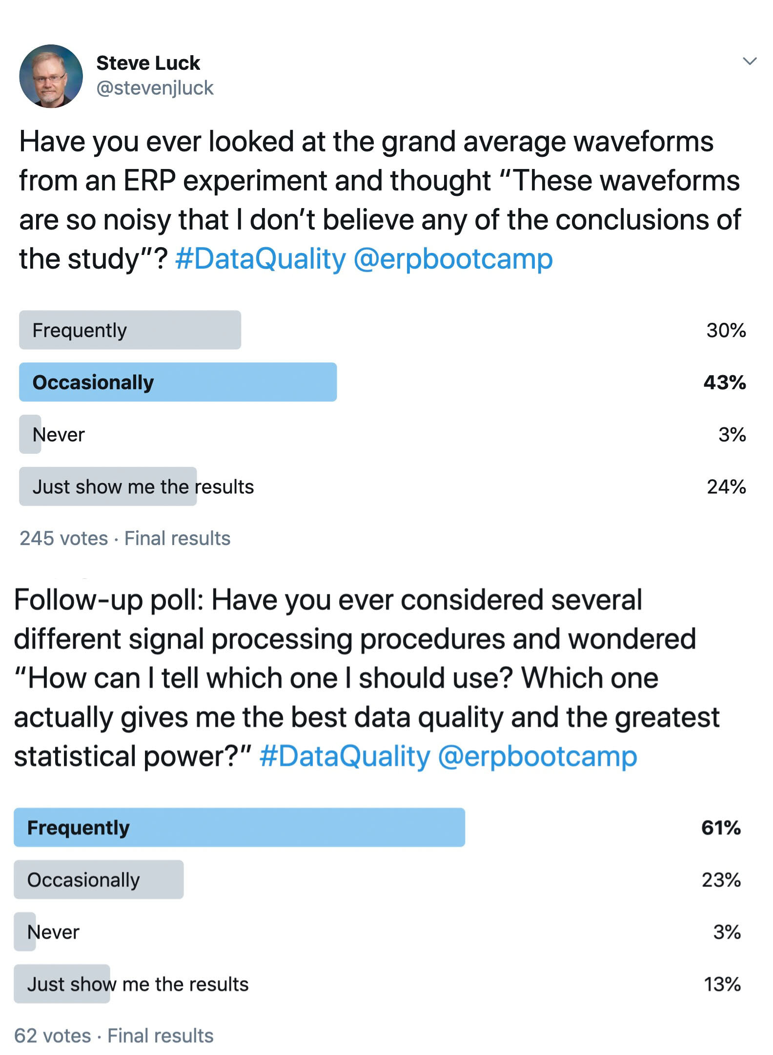
I’ve been doing ERP research for over 30 years, and for that entire time I have been looking for a metric of data quality. I’d like to be able to quantify the noise in my data in a variety of different paradigms, and I’d like to be able to determine exactly how a given signal processing operation (e.g., filtering) changes the signal-to-noise ratio of my data. And when I review a manuscript with really noisy-looking data, making me distrust the conclusions of the study, I’d like to be able to make an objective judgment rather than a subjective judgment. Given the results of the Twitter polls shown here, a lot of other people would also like to have a good metric of data quality.

I’ve looked around for such a metric for many years, but I never found one. So a few years ago, I decided that I should try to create one. I enlisted the aid of Andrew Stewart, Aaron Simmons, and Mijke Rhemtulla, and together we’ve developed a very simple but powerful and flexible metric of data quality that we call the Standardized Measurement Error or SME.

The SME has 3 key properties:

  1. It reflects the extent to which noise (i.e., trial-to-trial variations in the EEG recording) impacts the score that you are actually using as the dependent variable in your study (e.g., the peak latency of the P3 wave). This is important, because the effect of noise will differ across different amplitude and latency measures. For example, high-frequency noise will have a big impact on the peak amplitude between 300 and 500 ms but relatively little impact on the mean voltage during this time range. The impact of noise depends on both the nature of the noise and what you are trying to measure.

  2. It quantifies the data quality for each individual participant at each electrode site of interest, making it possible to determine (for example) whether a given participant’s data are so noisy that the participant should be excluded from the statistical analyses or whether a given electrode should be interpolated.

  3. It can be aggregated across participants in a way that allows you to estimate the impact of the noise on your effect sizes and statistical power and to estimate how your effect sizes and power would change if you increased or decreased the number of trials per participant.

The SME is a very simple metric: It’s just the standard error of measurement of the score of interest (e.g., the standard error of measurement for the peak latency value between 300 and 500 ms). It is designed to answer the question: If I repeated this experiment over and over again in the same participant (assuming no learning, fatigue, etc.), and I obtained the score of interest in each repetition, how similar would the scores be across repetitions? For example, if you repeated an experiment 10,000 times in a given participant, and you measured P3 peak latency for each of the 10,000 repetitions, you could quantify the consistency of the P3 peak latency scores by computing the standard deviation (SD) of the 10,000 scores. The SME metric provides a way of estimating this SD using the data you obtained in a single experiment with this participant.

The SME can be estimated for any ERP amplitude or latency score that is obtained from an averaged ERP waveform. If you quantify amplitude as the mean voltage across some time window (e.g., 300-500 ms for the P3 wave), the SME is trivial to estimate. If you want to quantify peak amplitude or peak latency, you can still use the SME, but it requires a somewhat more complicated estimation technique called bootstrapping. Bootstrapping is incredibly flexible, and it allows you to estimate the SME for very complex scores, such as the onset latency of the N2pc component in a contralateral-minus-ipsilateral difference wave.

Should you start using the SME to quantify data quality in your own research? Yes!!! Here are some things you could do if you had SME values:

  • Determine whether your data quality has increased or decreased when you modify a data analysis step or experimental design feature

  • Notice technical problems that are reducing your data quality (e.g., degraded electrodes, a poorly trained research assistant) 

  • Determine whether a given participant’s data are too noisy to be included in the analyses or whether a channel is so noisy that it should be replaced with interpolated values

  • Compare different EEG recording systems, different recording procedures, and different analysis pipelines to see which one yields the best data quality

The SME would be even more valuable if researchers started regularly including SME values in their publications. This would allow readers/reviewers to objectively assess whether the results are beautifully clean, unacceptably noisy, or somewhere in between. Also, if every ERP paper reported the SME, we could easily compare data quality across studies, and the field could determine which recording and analysis procedures produce the cleanest data. This would ultimately increase the number of true, replicable findings and decrease the number of false, unreplicable findings. 

My dream is that, 10 years from now, every new ERP manuscript I review and every new ERP paper I read will contain SME values (or perhaps some newer, better measure of data quality that someone else will be inspired to develop).

To help make that dream come true, we’re doing everything we can to make it easy for people to compute SME values. We’ve just released a new version of ERPLAB Toolbox (v8.0) that will automatically compute the SME using default time windows every time you make an averaged ERP waveform. These SME values will be most appropriate when you are scoring the amplitude of an ERP component as the mean voltage during some time window (e.g., 300-500 ms for the P3 wave), but they also give you an overall sense of your data quality.  If you are using some other method to score your amplitudes or latencies (e.g., peak latency), you will need to write a simple Matlab script that uses bootstrapping to estimate the SME. However, we have provided several example scripts, and anyone who knows at least a little bit about Matlab scripting should be able to adapt our scripts for their own data. And we hope to add an automated method for bootstrapping in future versions of ERPLAB.

By now, I’m sure you’ve decided you want to give it a try, and you’re wondering where you can get more information.  Here are links to some useful resources:

On the application of decoding/classification/MVPA approaches to ERP data

If you pay any attention to the fMRI literature, you know that there has been a huge increase in the number of studies applying multivariate methods to the pattern of voxels (as opposed to univariate methods that examine the average activity over a set of voxels). For example, if you ask whether the pattern of activity across the voxels within a given region is different for faces versus objects, you’ll find that many areas carry information about whether a stimulus is a face or an object even if the overall activity level is no different for faces versus objects. This class of methods goes by several different names, including multivariate pattern analysis (MVPA), classification, and decoding. I will use the term decoding here, but I am treating these terms as if they are equivalent.

Gi-Yeul Bae and I have recently started applying decoding methods to sustained ERPs and to EEG oscillations (see this paper and this more recent paper), and others have also used them (especially in the brain-computer interface [BCI] field). We have found that decoding can pick up on incredibly subtle signals that would be missed by conventional methods, and I believe that decoding methods have the potential to open up new areas of ERP research, allowing us to answer questions that would ordinarily seem impossible (just as has happened in the fMRI literature). The goal of this blog post is to provide a brief introduction so that you can more easily read papers using these methods and can apply them to your own research.

There are many ways to apply decoding to EEG/ERP data, and I will focus on the approach that we have been using to study perception, attention, and working memory. Our goal in using decoding methods is to determine what information about a stimulus is represented in the brain at a given moment in time, and we apply decoding to averaged ERP waveforms to minimize noise and maximize our ability to detect subtle neural signals. This is very different from the BCI literature, where the goal is to reliably detect signals on single trials that can be used to control devices in real time.

To explain our approach, I will give a simple but hypothetical example. Our actual research examines much more complex situations, so this hypothetical example will be clearer. In this hypothetical study, we present subjects with a sequence 180 face photographs and 180 car photographs, asking them to simply press a single button for each stimulus. A conventional analysis will yield a larger N170 component for the faces than for the cars, especially over lateral occipitotemporal cortex.

Our decoding approach asks, for each individual subject, whether we can reliably predict whether the stimuli that generated a given ERP waveform were faces or cars. To do this, we will take the 180 face trials and the 180 car trials for a given subject and randomly divide them into 3 sets of 60 trials. This will give us 3 averaged face ERP waveforms and 3 averaged car ERP waveforms. We will then take 2 of the face waveforms and two of the car waveforms and feed them into a support vector machine (SVM), which is a powerful machine learning algorithm. The SVM “learns” how the face and car ERPs differ. We do this separately at each time point, feeding the SVM for that time point the voltage from each electrode site at that time point. In other words, the SVM learns how the scalp distribution for the face ERP differs from the scalp distribution for the car ERP at that time point (for a single subject). We then take the scalp distribution at this point in time from the 1 face ERP and the 1 car ERP that were not used to train the SVM, and we ask whether the SVM can correctly guess whether each of these scalp distributions is from a face ERP or a house ERP. We then repeat this process over and over many times using different subsets of trials to create the averaged ERPs used for training and for testing. We can then ask whether, over these many iterations, the SVM can guess whether the test ERP is from faces or cars above chance (50% correct).

This process is applied separately for each time point and separately for each subject, giving us a classification accuracy value for each subject at each time point (see figure below, which shows imaginary data from this hypothetical experiment). We then aggregate across subjects, yielding a waveform showing average classification accuracy at each time point, and we use the mass univariate approach to find clusters of time points at which the accuracy is significantly greater than chance.

Decoding Example.jpg

In some sense, the decoding approach is the mirror image of the conventional approach. Instead of asking whether the face and car waveforms are significantly different at a given point in time, we are asking whether we can predict whether the waveforms come from faces or cars at a given point in time significantly better than chance. However, there are some very important practical differences between the decoding approach and the conventional approach. First, and most important, the decoding is applied separately to each subject, and we aggregate across subjects only after computing %correct. As a result, the decoding approach picks up on the differences between faces and cars at whatever electrode sites show a difference in a particular subject. By contrast, the conventional approach can find differences between faces and cars only to the extent that subjects have similar effects. Given that there are often enormous differences among subjects, the single-subject decoding approach can give us much greater power to detect subtle effects. A second difference is that the SVM effectively “figures out” the pattern of scalp differences that most optimally differentiates between faces and cars. That is, it uses the entire scalp distribution in a very intelligent way. This can also give us greater power to detect subtle effects.

In our research so far, we have been able to detect very subtle effects that never would have been statistically significant in conventional analyses. For example, we can determine which of 16 orientations is being held in working memory at a given point in time (see this paper), and we can determine which of 16 directions of motion is currently being perceived (see this paper). We can even decode the orientation that was presented on the previous trial, even though it’s no longer task relevant (see here). We have currently-unpublished data showing that we can decode face identity and facial expression, the valence and arousal of emotional scenes from the IAPS database, and letters of the alphabet (even when presented at 10 per second).

You can also use decoding to study between-group differences. Some research uses decoding to try to predict which group an individual belongs to (e.g., a patient group or a control group). This can be useful for diagnosis, but it doesn’t usually provide much insight into how the brain activity differs between groups. Our approach has been to use decoding to ask about the nature of the neural representations within each group. But this can be tricky, because decoding is highly sensitive to the signal-to-noise ratio, which may differ between groups for “uninteresting” reasons (e.g., more movement artifacts in one group). We have addressed these issues in this study that compares decoding accuracy in people with schizophrenia and matched control subjects.

How to p-hack (and avoid p-hacking) in ERP Research

Luck, S. J., & Gaspelin, N. (2017). How to Get Statistically Significant Effects in Any ERP Experiment (and Why You Shouldn’t)Psychophysiology, 54, 146-157.

Figure 3b.jpg

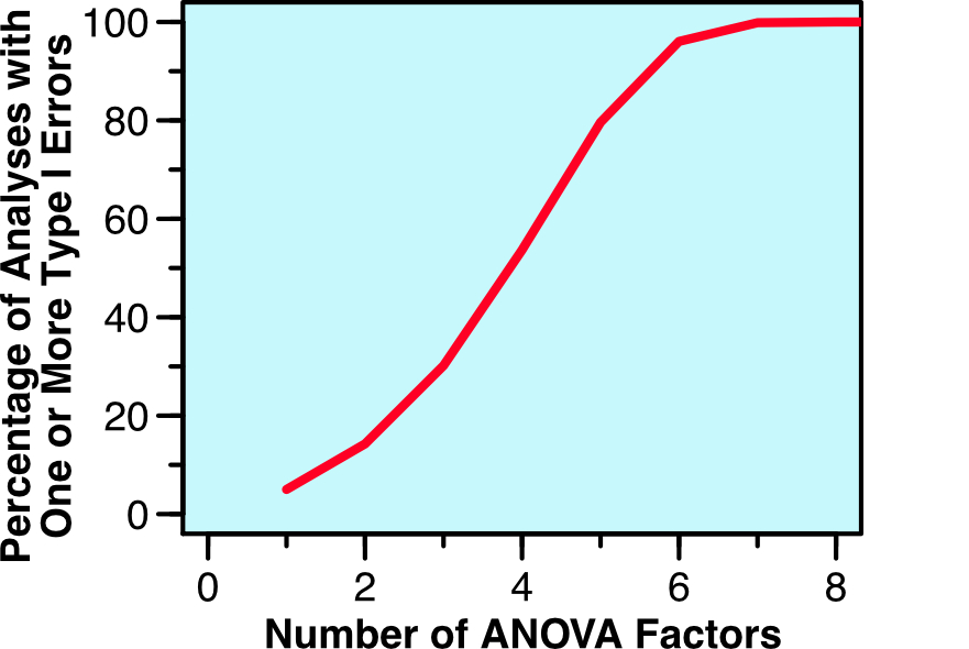
In this article, we show how ridiculously easy it is to find significant effects in ERP experiments by using the observed data to guide the selection of time windows and electrode sites. We also show that including multiple factors in your ANOVAs can dramatically increase the rate of false positives (Type I errors). We provide some suggestions for methods to avoid inflating the Type I error rate.

This paper was part of a special issue of Psychophysiology on Reproducibility edited by Emily Kappenman and Andreas Keil.