Step-by-Step Protocols for Collecting Clean EEG Data

Standard Version: Farrens, J. L., Simmons, A. M., Luck, S. J., & Kappenman, E. S. (2019). Electroencephalogram (EEG) Recording Protocol for Cognitive and Affective Human Neuroscience Research. Protocol Exchange. https://doi.org/10.21203/rs.2.18328/v2 [PDF]

COVID-19 Version: Simmons, A. M., & Luck, S. J. (2020). Protocol for Reducing COVID-19 Transmission Risk in EEG Research. Protocol Exchange. https://doi.org/10.21203/rs.3.pex-974/v2

We have published an in-depth description of our EEG recording procedures, which provides an extremely detailed, step-by-step account of how we currently record EEG data in our laboratories (along with a modified version to minimize risk of COVID-19 transmission). Although this level of detail important for collecting clean data, it would be unrealistic to include 20+ pages of recording details in the Method section of a journal article. By publishing this protocol and then citing it in our papers, other researchers will know exactly how we recorded our data, which will enhance reproducibility. In addition, this protocol provides a forum for sharing the tips and tricks we have developed for collecting clean EEG data, which may help you improve your data quality. We encourage other researchers to either follow and cite our protocol or publish and cite their own protocols. If you’d like more information about why we think this is important, read on…

If you’ve ever recorded or processed raw EEG data, you know how noisy the data can be. The neural signals we want to record are contaminated by a variety of biological and non-biological noise sources, including muscle activity (EMG), heartbeats (EKG), skin potentials, movement artifacts, and induced electrical noise from the environment. To maximize the likelihood of finding the neural effects of interest, researchers need to do everything they can to reduce the noise during a recording session. Postprocessing techniques such as filters can help, but they can’t eliminate all the noise, and they often have a cost (e.g., temporal distortion). This is why one of our ERP Boot Camp mottos is “There is no substitute for clean data!”

When you run an EEG recording session, there are a million little details that together impact the quality of the data. Every lab has its own approach, but our field has no widely used mechanism for sharing these methodological details. Recording methods are usually described in journal articles with only a brief mention of the recording parameters (e.g., filter settings and sampling rate) and no information about the millions of other details that impact data quality. And really, who would want to slog through a Method section that described how the electrodes were oriented in their holders or listed the specific make and model of chair that was used to ensure that the participant remained comfortable?

However, these details really matter. For example, we have shown that the temperature of the recording environment can have a substantial impact on statistical power (Kappenman & Luck, 2010), but we have never seen an EEG/ERP paper from another lab that mentioned the temperature of the recording room.

A mechanism now exists for reporting all of these details. Specifically, one can now easily publish a formal protocol that is permanent and citable (and even contributes to citation counts on Google Scholar, if you care about that sort of thing). There are a variety of ways to publish a protocol, but we chose Nature’s Protocol Exchange web site. It’s free, appears to be robust, and automatically generates a DOI. It does not involve peer review (because you are merely listing your procedures, not drawing any formal conclusions), but it does involve a quick administrative review (to make sure that inappropriate materials are not posted). The protocol is published with a Creative Commons license, so Nature does not own it, and anyone can use it. Other sites may be even better, but Protocol Exchange fits our current needs reasonably well (although we would have appreciated a little more control over the formatting).

We encourage other researchers to read our protocol and use it to get ideas for their own recording methods. Our methods may not be ideal for some kinds of research, and other labs may have equivalent or even better methods.

More than anything, we hope that our protocol inspires other researchers to start publishing their own detailed protocols. This sharing of information will help everyone collect the cleanest possible data, improving the quality of published research in our field. Detailed protocols will also increase reproducibility of research methods and perhaps even replicability of research findings. Note that our protocol is longer and more detailed that what most labs would publish (because we included advice about things like fixing broken electrodes).

You can find the standard version of the protocol at protocolexchange.researchsquare.com/article/663a5a19-c74e-4c7d-b3fc-9c5188332b46/v2 or at doi.org/10.21203/rs.2.18328/v2. You can download a nicely formatted PDF of the protocol here.

You can find the COVID-19 version at https://protocolexchange.researchsquare.com/article/pex-974/v2 or at https://doi.org/10.21203/rs.3.pex-974/v2

Why experimentalists should ignore reliability and focus on precision

It is commonly said that “a measure cannot be valid if it is not reliable.” It turns out that this is not true as these terms are typically defined in psychology. And it also turns out that, although reliability is extremely important in some types of research (e.g., correlational studies of individual differences), it’s the wrong way for most experimentalists to think about the quality of their measures.

I’ve been thinking about this issue for the last 2 years, as my lab has been working on a new method for quantifying data quality in ERP experiments (stay tuned for a preprint). It turns out that ordinary measures of reliability are quite unsatisfactory for assessing whether ERP data are noisy. This is also true for reaction time (RT) data. A couple days ago, Michaela DeBolt (@MDeBoltC) alerted me to a new paper by Hedge et al. (2018) showing that typical measures of reliability can be low even when power is high in experimental studies. There’s also a recent paper on MRI data quality by Brandmaier et al. (2018) that includes a great discussion of how the term “reliability” is used to mean different things in different fields.

Here’s a quick summary of the main issue: Psychologists usually quantify reliability using correlation-based measures such as Cronbach’s alpha. Because the magnitude of a correlation depends on the amount of true variability among participants, these measures of reliability can go up or down a lot depending on how homogeneous the population is. All else being equal, a correlation will be lower if the participants are more homogeneous. Thus, reliability (as typically quantified by psychologists) depends on the range of values in the population being tested as well as the nature of the measure. That’s like a physicist saying that the reliability of a thermometer depends on whether it is being used in Chicago (where summers are hot and winters are cold) or in San Diego (where the temperature hovers around 72°F all year long).

One might argue that this is not really what psychometricians mean when they’re talking about reliability (see Li, 2003, who effectively redefines the term “reliability” to capture what I will be calling “precision”). However, the way I will use the term “reliability” captures the way this term has been operationalized in 100% of the papers I have read that have quantified reliability (and in the classic texts on psychometrics cited by Li, 2003).

A Simple Reaction Time Example

Let’s look at this in the context of a simple reaction time experiment. Imagine that two researchers, Dr. Careful and Dr. Sloppy, use exactly the same task to measure mean RT (averaged over 50 trials) from each person in a sample of 100 participants (drawn from the same population). However, Dr. Careful is meticulous about reducing sources of extraneous variability, and every participant is tested by an experienced research assistant at the same time of day (after a good night’s sleep) and at the same time since their last meal. In contrast, Dr. Sloppy doesn’t worry about these sources of variance, and the participants are tested by different research assistants at different times of day, with no effort to control sleepiness or hunger. The measures should be more reliable for Dr. Careful than for Dr. Sloppy, right? Wrong! Reliability (as typically measured by psychologists) will actuallybe higher for Dr. Sloppy than for Dr. Careful (assuming that Dr. Sloppy hasn’t also increased the trial-to-trial variability of RT).

To understand why this is true, let’s take a look at how reliability would typically be quantified in a study like this. One common way to quantify the reliability of the RT measure is the split-half reliability. (There are better measures of reliability, but they all lead to the same problem, and split-half reliability is easy to explain.) To compute the split-half reliability, the researchers divide the trials for each participant into odd-numbered and even-numbered trials, and they calculate the mean RT separately for the odd- and even-numbered trials. This gives them two values for each participant, and they simply compute the correlation between these two values. The logic is that, if the measure is reliable, then the mean RT for the odd-numbered trials should be pretty similar to the mean RT for the even-numbered trials in a given participant, so individuals with a fast mean RT for the odd-numbered trials should also have a fast mean RT for the even-numbered trials, leading to a high correlation. If the measure is unreliable, however, the mean RTs for the odd- and even-numbered trials will often be quite different for a given participant, leading to a low correlation.

However, correlations are also impacted by the range of scores, and the correlation between the mean RT for the odd- versus even-numbered trials will end up being greater for Dr. Sloppy than for Dr. Careful because the range of mean RTs is greater for Dr. Sloppy (e.g., because some of Dr. Sloppy’s participants are sleepy and others are not). This is illustrated in the scatterplots below, which show simulations of the two experiments. The experiments are identical in terms of the precision of the mean RT measure (i.e., the trial-to-trial variability in RT for a given participant). The only thing that differs between the two simulations is the range of true mean RTs (i.e., the mean RT that a given participant would have if there were no trial-by-trial variation in RT). Because all of Dr. Careful’s participants have mean RTs that cluster closely around 500 ms, the correlation between the mean RTs for the odd- and even-numbered trials is not very high (r=.587). By contrast, because some of Dr. Sloppy’s participants are fast and others are slow, the correlation is quite good (r=.969). Thus, simply by allowing the testing conditions to vary more across participants, Dr. Sloppy can report a higher level of reliability than Dr. Careful. 

Reliability and Precision.jpg

Keep in mind that Dr. Careful and Dr. Sloppy are measuring mean RT in exactly the same way. The actual measure is identical in their studies, and yet the measured reliability differs dramatically across the studies because of the differences in the range of scores. Worse yet, the sloppy researcher ends up being able to report higher reliability than the careful researcher.

Let’s consider an even more extreme example, in which the population is so homogeneous that every participant would have the same mean RT if we averaged together enough trials, and any differences across participants in observed mean RT are entirely a result of random variation in single-trial RTs. In this situation, the split-half reliability would have an expected value of zero. Does this mean that mean RT is no longer a valid measure of processing speed? Of course not—our measure of processing speed is exactly the same in this extreme case as in the studies of Dr. Careful and Dr. Sloppy. Thus, a measure can be valid even if it is completely unreliable (as typically quantified by psychologists).

Here’s another instructive example. Imagine that Dr. Careful does two studies, one with a population of college students at an elite university (who are relatively homogeneous in age, education, SES, etc.) and one with a nationally representative population of U.S. adults (who vary considerably in age, education, SES, etc.). The range of mean RT values will be much greater in the nationally representative population than in the college student population. Consequently, even if Dr. Careful runs the study in exactly the same way in both populations, the reliability will likely be much greater in the nationally representative population than in the college student population. Thus, reliability (as typically measured by psychologists) depends on the range of scores in the population being measured and not just on the properties of the measure itself. This is like saying that a thermometer is more reliable in Chicago than in San Diego simply because the range of temperatures is greater in Chicago.

Example of an Experimental Manipulation

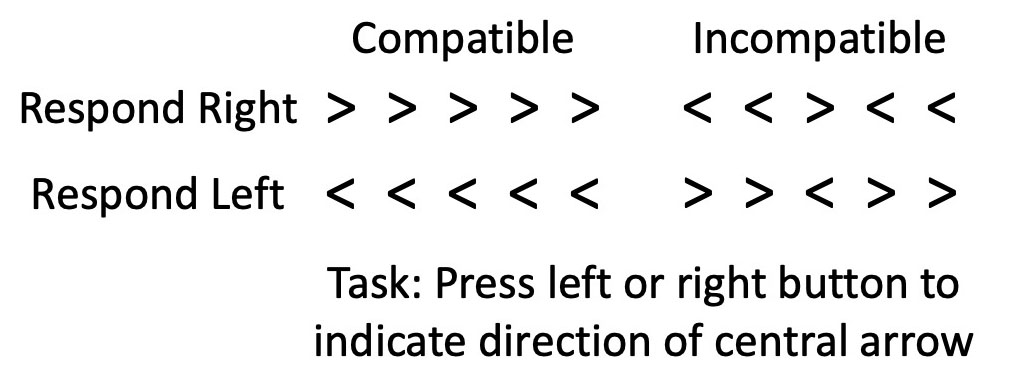
Flankers.jpg

Now let’s imagine that Dr. Careful and Dr. Sloppy don’t just measure mean RT in a single condition, but they instead test the effects of a within-subjects experimental manipulation. Let’s make this concrete by imagining that they conduct a flankers experiment, in which participants report whether a central arrow points left or right while ignoring flanking stimuli that are either compatible or incompatible with the central stimulus (see figure to the right). In a typical study, mean RT would be slowed on the incompatible trials relative to the compatible trials (a compatibility effect).

If we look at the mean RTs in a given condition of this experiment, we will see that the mean RT varies from participant to participant much more in Dr. Sloppy’s version of the experiment than in Dr. Careful’s version (because there is more variation in factors like sleepiness in Dr. Sloppy’s version). Thus, as in our original example, the split-half reliability of the mean RT for a given condition will again be higher for Dr. Sloppy than for Dr. Careful. But what about the split-half reliability of the flanker compatibility effect? We can quantify the compatibility effect as the difference in mean RT between the compatible and incompatible trials for a given participant, averaged across left-response and right-response trials. (Yes, there are better ways to analyze these data, but they all lead to the same conclusions about reliability.) We can compute the split-half reliability of the compatibility effect by computing it twice for every subject—once for the odd-numbered trials and once for the even-numbered trials—and calculating the correlation between these values.

The compatibility effect, like the raw RT, is likely to vary according to factors like the time of day, so the range of compatibility effects will be greater for Dr. Sloppy than for Dr. Careful. And this means that the split-half reliability will again be greater for Dr. Sloppy than for Dr. Careful. (Here I am assuming that trial-to-trial variability in RT is not impacted by the compatibility manipulation and by the time of day, which might not be true, but nonetheless it is likely that the reliability will be at least as high for Dr. Sloppy as for Dr. Careful.)

By contrast, statistical power for determining whether a compatibility effect is present will be greater for Dr. Careful than for Dr. Sloppy. In other words, if we use a one-sample t test to compare the mean compatibility effect against zero, the greater variability of this effect in Dr. Sloppy’s experiment will reduce the power to determine whether a compatibility effect is present. So, even though reliability is greater for Dr. Sloppy than for Dr. Careful, statistical power for detecting an experimental effect is greater for Dr. Careful than for Dr. Sloppy. If you care about statistical power for experimental effects, reliability is probably not the best way for you to quantify data quality.

An Example of Individual Differences

What if Dr. Careful and Dr. Sloppy wanted to look at individual differences? For example, imagine that they were testing the hypothesis that the flanker compatibility effect is related to working memory capacity. Let’s assume that they measure both variables in a single session. Assuming that both working memory capacity and the compatibility effect vary as a function of factors like time of day, Dr. Sloppy will find greater reliability for both working memory capacity and the compatibility effect (because the range of values is greater for both variables in Dr. Sloppy’s study than in Dr. Careful’s study). Moreover, the correlation between working memory capacity and the compatibility effect will be higher in Dr. Sloppy’s study than in Dr. Careful’s study (again because of differences in the range of scores).

In this case, greater reliability is associated with stronger correlations, just as the psychometricians have always told us. All else being equal, the researcher who has greater reliability for the individual measures (Dr. Sloppy in this example) will find a greater correlation between them. So, if you want to look at correlations between measures, you want to maximize the range of scores (which will in turn maximize your reliability). However, recall that Dr. Careful had more statistical power than Dr. Sloppy for detecting the compatibility effect. Thus, the same factors that increase reliability and correlations between measures can end up reducing statistical power when you are examining experimental effects with exactly the same measures. (Also, if you want to look at correlations between RT and other measures, I recommend that you read Miller & Ulrich, 2013, which shows that these correlations are more difficult to interpret than you might think.)

It’s also important to note that Dr. Sloppy would run into trouble if we looked at test-retest reliability instead of split-half reliability. That is, imagine that Dr. Sloppy and Dr. Careful run studies in which each participant is tested on two different days. Dr. Careful makes sure that all of the testing conditions (e.g., time of day) are the same for every participant, but Dr. Sloppy isn’t careful to keep the testing conditions constant between the two session for each participant. The test-retest reliability (the correlation between the measure on Day 1 and Day 2) would be low for Dr. Sloppy. Interestingly, Dr. Sloppy would have high split-half reliability (because of the broad range of scores) but poor test-retest reliability. Dr. Sloppy would also have trouble if the compatibility effect and working memory capacity were measured on different days.

Precision vs. Reliability

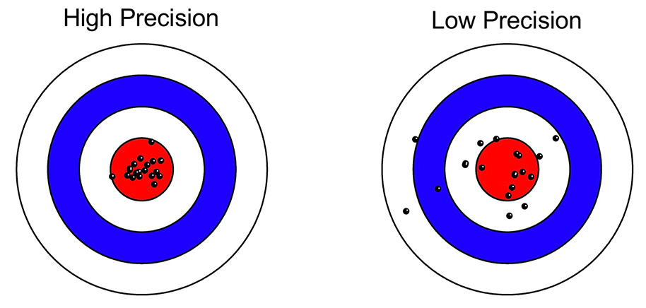
Now let’s turn to the distinction between reliability and precision. The first part of the Brandmaier et al. (2018) paper has an excellent discussion of how the term “reliability” is used differently across fields. In general, everyone agrees that a measure is reliable to the extent that you get the same thing every time you measure it. The difference across fields lies in how reliability is quantified. When we think about reliability in this way, a simple way to quantify it would be to obtain the measure a large number of times under identical conditions and compute the standard deviation (SD) of the measurements. The SD is a completely straightforward measure of the “the extent that you get the same thing every time you measure it.” For example, you could use a balance to weigh an object 100 times, and the standard deviation of the weights would indicate the reliability of the balance. Another term for this would be the “precision” of the balance, and I will use the term “precision” to refer to the SD over multiple measurements. (In physics, the SD is typically divided by the mean to get the coefficient of variability, which is often a better way to quantify reliability for measures like weight that are on a ratio scale.)

The figure below (from the Brandmaier article) shows what is meant by low and high precision in this context, and you can see how the SD would be a good measure of precision. The key is that precision reflects the variability of the measure around its mean, not whether the mean is the true mean (which would be the accuracy or bias of the measure).

Precision from Brandmaier 2018.jpg

Things are more complicated in most psychology experiments, where there are (at least) two distinct sources of variability in a given experiment: true differences among participants (called the true score variance) and measurement imprecision. However, in a typical experiment, it is not obvious how to separately quantify the true score variance from the measurement imprecision. For example, if you measure a dependent variable once from N participants, and you look at the variance of those values, the result will be the sum of the true score variance and the variance due to measurement error. These two sources of variance are mixed together, and you don’t know how much of the variance is a result of measurement imprecision.

Imagine, however, that you’ve measured the dependent variable twice from each subject. Now you could ask how close the two measures are to each other. For example, if we take our original simple RT experiment, we could get the mean RT from the odd-number trials and the mean RT from the even-numbered trials in each participant. If these two scores were very close to each other in each participant, then we would say we have a precise measure of mean RT. For example, if we collected 2000 trials from each participant, resulting in 1000 odd-numbered trials and 1000 even-numbered trials, we’d probably find that the two mean RTs for a given subject were almost always within 10 ms of each other. However, if collected only 20 trials from each participant, we would see big differences between the mean RTs from the odd- and even-numbered trials. This makes sense: All else being equal, mean RT should be a more precise measure if it’s based on more trials.

In a general sense, we’d like to say that mean RT is a more reliable measure when it’s based on more trials. However, as the first part of this blog post demonstrated, typical psychometric approaches to quantifying reliability are also impacted by the range of values in the population and not just the precision of the measure itself: Dr. Sloppy and Dr. Careful were measuring mean RT with equal precision, but split-half reliability was greater for Dr. Careful than for Dr. Sloppy because there was a greater range of mean RT values in Dr. Sloppy’s study. This is because split-half reliability does not look directly at how similar the mean RTs are for the odd- and even-numbered trials; instead, it involves computing the correlation between these values, which in turn depends on the range of values across participants.

How, then, can we formally quantify precision in a way that does not depend on the range of values across participants? If we simply took the difference in mean RT between the odd- and even-numbered trials, this score would be positive for some participants and negative for others. As a result, we can’t just average this difference across participants. We could take the absolute value of the difference for each participant and then average across participants, but absolute values are problematic in other ways. Instead, we could just take the standard deviation (SD) of the two scores for each person. For example, if Participant #1 had a mean RT of 515 ms for the odd-numbered trials and a mean RT of 525 ms for the even-numbered trials, the SD for this participant would be 7.07 ms. SD values are always positive, so we could average the single-participant SD values across participants, and this would give us an aggregate measure of the precision of our RT measure.

The average of the single-participant SDs would be a pretty good measure of precision, but it would underestimate the actual precision of our mean RT measure. Ultimately, we’re interested in the precision of the mean RT for all of the trials, not the mean RT separately for the odd- and even-numbered trials. By cutting the number of trials in half to get separate mean RTs for the odd- and even-numbered trials, we get an artificially low estimate of precision.

Fortunately, there is a very familiar statistic that allows you to quantify the precision of the mean RT using all of the trials instead of dividing them into two halves. Specifically, you can simply take all of the single-trial RTs for a given participant in a given condition and compute the standard error of the mean (SEM). This SEM tells you what you would expect to find if you computed the mean RT for that subject in each of an infinite number of sessions and then took the SD of the mean RT values.

Let’s unpack that. Imagine that you brought a single participant to the lab 1000 times, and each time you ran 50 trials and took the mean RT of those 50 trials. (We’re imagining that the subject’s performance doesn’t change over repeated sessions; that’s not realistic, of course, but this is a thought experiment so it’s OK.) Now you have 1000 mean RTs (each based on the average of 50 trials). You could take the SD of those 1000 mean RTs, and that would be an accurate way of quantifying the precision of the mean RT measure. It would be just like a chemist who weighs a given object 1000 times on a balance and then uses the SD of these 1000 measurements to quantify the precision of the balance.

But you don’t actually need to bring the participant to the lab 1000 times to estimate the SD. If you compute the SEM of the 50 single-trial RTs in one session, this is actually an estimate of what would happen if you measured mean RT in an infinite number of sessions and then computed the SD of the mean RTs. In other words, the SEM of the single-trial RTs in one session is an estimate of the SD of the mean RT across an infinite number of sessions. (Technical note: It would be necessary to deal with the autocorrelation of RT across trials, but there are methods for that.)

Thus, you can use the SEM of the single-trial RTs in a given session as a measure of the precision of the mean RT measure for that session. This gives you a measure of the precision for each individual participant, and you can then just average these values across participants. Unlike traditional measures of reliability, this measure of precision is completely independent of the range of values across the population. If Dr. Careful and Dr. Sloppy used this measure of precision, they would get exactly the same value (because they’re using exactly the same procedure to measure mean RT in a given participant). Moreover, this measure of precision is directly related to the statistical power for detecting differences between conditions (although there is a trick for aggregating the SEM values across participants, as will be detailed in our paper on ERP data quality).

So, if you want to assess the quality of your data in an experimental study, you should compute the SEM of the single-trial values for each subject, not some traditional measure of “reliability.” Reliability is very important for correlational studies, but it’s not the right measure of data quality in experimental studies.

Here’s the bottom line: the idea that “a measure cannot be valid if it is not reliable” is not true for experimentalists (given how reliability is typically operationalized by psychologists), and they should focus on precision rather than reliability.

On the application of decoding/classification/MVPA approaches to ERP data

If you pay any attention to the fMRI literature, you know that there has been a huge increase in the number of studies applying multivariate methods to the pattern of voxels (as opposed to univariate methods that examine the average activity over a set of voxels). For example, if you ask whether the pattern of activity across the voxels within a given region is different for faces versus objects, you’ll find that many areas carry information about whether a stimulus is a face or an object even if the overall activity level is no different for faces versus objects. This class of methods goes by several different names, including multivariate pattern analysis (MVPA), classification, and decoding. I will use the term decoding here, but I am treating these terms as if they are equivalent.

Gi-Yeul Bae and I have recently started applying decoding methods to sustained ERPs and to EEG oscillations (see this paper and this more recent paper), and others have also used them (especially in the brain-computer interface [BCI] field). We have found that decoding can pick up on incredibly subtle signals that would be missed by conventional methods, and I believe that decoding methods have the potential to open up new areas of ERP research, allowing us to answer questions that would ordinarily seem impossible (just as has happened in the fMRI literature). The goal of this blog post is to provide a brief introduction so that you can more easily read papers using these methods and can apply them to your own research.

There are many ways to apply decoding to EEG/ERP data, and I will focus on the approach that we have been using to study perception, attention, and working memory. Our goal in using decoding methods is to determine what information about a stimulus is represented in the brain at a given moment in time, and we apply decoding to averaged ERP waveforms to minimize noise and maximize our ability to detect subtle neural signals. This is very different from the BCI literature, where the goal is to reliably detect signals on single trials that can be used to control devices in real time.

To explain our approach, I will give a simple but hypothetical example. Our actual research examines much more complex situations, so this hypothetical example will be clearer. In this hypothetical study, we present subjects with a sequence 180 face photographs and 180 car photographs, asking them to simply press a single button for each stimulus. A conventional analysis will yield a larger N170 component for the faces than for the cars, especially over lateral occipitotemporal cortex.

Our decoding approach asks, for each individual subject, whether we can reliably predict whether the stimuli that generated a given ERP waveform were faces or cars. To do this, we will take the 180 face trials and the 180 car trials for a given subject and randomly divide them into 3 sets of 60 trials. This will give us 3 averaged face ERP waveforms and 3 averaged car ERP waveforms. We will then take 2 of the face waveforms and two of the car waveforms and feed them into a support vector machine (SVM), which is a powerful machine learning algorithm. The SVM “learns” how the face and car ERPs differ. We do this separately at each time point, feeding the SVM for that time point the voltage from each electrode site at that time point. In other words, the SVM learns how the scalp distribution for the face ERP differs from the scalp distribution for the car ERP at that time point (for a single subject). We then take the scalp distribution at this point in time from the 1 face ERP and the 1 car ERP that were not used to train the SVM, and we ask whether the SVM can correctly guess whether each of these scalp distributions is from a face ERP or a house ERP. We then repeat this process over and over many times using different subsets of trials to create the averaged ERPs used for training and for testing. We can then ask whether, over these many iterations, the SVM can guess whether the test ERP is from faces or cars above chance (50% correct).

This process is applied separately for each time point and separately for each subject, giving us a classification accuracy value for each subject at each time point (see figure below, which shows imaginary data from this hypothetical experiment). We then aggregate across subjects, yielding a waveform showing average classification accuracy at each time point, and we use the mass univariate approach to find clusters of time points at which the accuracy is significantly greater than chance.

Decoding Example.jpg

In some sense, the decoding approach is the mirror image of the conventional approach. Instead of asking whether the face and car waveforms are significantly different at a given point in time, we are asking whether we can predict whether the waveforms come from faces or cars at a given point in time significantly better than chance. However, there are some very important practical differences between the decoding approach and the conventional approach. First, and most important, the decoding is applied separately to each subject, and we aggregate across subjects only after computing %correct. As a result, the decoding approach picks up on the differences between faces and cars at whatever electrode sites show a difference in a particular subject. By contrast, the conventional approach can find differences between faces and cars only to the extent that subjects have similar effects. Given that there are often enormous differences among subjects, the single-subject decoding approach can give us much greater power to detect subtle effects. A second difference is that the SVM effectively “figures out” the pattern of scalp differences that most optimally differentiates between faces and cars. That is, it uses the entire scalp distribution in a very intelligent way. This can also give us greater power to detect subtle effects.

In our research so far, we have been able to detect very subtle effects that never would have been statistically significant in conventional analyses. For example, we can determine which of 16 orientations is being held in working memory at a given point in time (see this paper), and we can determine which of 16 directions of motion is currently being perceived (see this paper). We can even decode the orientation that was presented on the previous trial, even though it’s no longer task relevant (see here). We have currently-unpublished data showing that we can decode face identity and facial expression, the valence and arousal of emotional scenes from the IAPS database, and letters of the alphabet (even when presented at 10 per second).

You can also use decoding to study between-group differences. Some research uses decoding to try to predict which group an individual belongs to (e.g., a patient group or a control group). This can be useful for diagnosis, but it doesn’t usually provide much insight into how the brain activity differs between groups. Our approach has been to use decoding to ask about the nature of the neural representations within each group. But this can be tricky, because decoding is highly sensitive to the signal-to-noise ratio, which may differ between groups for “uninteresting” reasons (e.g., more movement artifacts in one group). We have addressed these issues in this study that compares decoding accuracy in people with schizophrenia and matched control subjects.

ERP Boot Camp Tip: Why mean amplitude is usually superior to peak amplitude

Traditionally, ERP amplitudes were quantified (scored) by finding the maximum voltage (or minimum voltage for a negative component) within some time period.  Why? Mainly because this was easy to do with a ruler and a pencil when your EEG system did not include a general-purpose computer and just gave you a printout of the waveform. When computers became available, and could easily quantify components in more sophisticated ways, many researchers continued to use peaks.

However, other researchers began scoring component amplitudes using the mean voltage within a particular time range. This is still far from perfect, but over time it has become clear that this mean amplitude approach had many advantages over peak amplitude. And there has been a clear shift toward the use of mean amplitude instead of peak amplitude.  However, peak amplitude is still used more than it should be.  The goal of this blog post is to describe some of the reasons why mean amplitude is usually preferable to peak amplitude so that researchers will make an informed choice and not just follow a tradition. A more detailed discussion is provided in Chapter 9 of An Introduction to the Event-Related Potential Technique, 2nd Edition (MIT Press). That chapter also discusses why peak latency is a poor measure of timing and describes some better alternatives.

Reason 1: Peaks and components are not the same thing.  Generally speaking, there's nothing special about the time at which the voltage reaches a maximum amplitude.  Given that multiple components are almost always overlapping at any given moment in time, the time and amplitude of the peak voltage will often not be the same as the time and amplitude of the peak of the component of interest.  Moreover, computational models of cognitive and neural processes rarely have much to say about when a process "peaks."  Instead, they focus on when a process begins, ends, etc.  So, peaks aren't particularly meaningful theoretically, and they can encourage an overly simplistic view of the relationship between the underlying components and the observed waveform.

Reason 2: Peak amplitude is typically less reliable than mean amplitude.  Peak amplitude is easily influenced by noise, whereas mean amplitude essentially filters out noise at high and intermediate frequencies. Here's a nice study showing that mean amplitude provides more robust results than peak amplitude: Clayson, P. E., Baldwin, S. A., & Larson, M. J. (2013). How does noise affect amplitude and latency measurement of event-related potentials (ERPs)? A methodological critique and simulation study. Psychophysiology, 50, 174-186.

Reason 3: The peak occurs at different times at different electrode sites.  An ERP component in the brain will have the same timing at every electrode site, but the timing of the peak voltage may differ considerably from site to site (because of other overlapping components). Consequently, when you measure the peak at multiple electrode sites, you're measuring the underlying component at different time points at each site, which is just a weird thing to do. More formally, it's not legitimate to look at the scalp distribution of a peak amplitude measurement (unless you find the peak at one electrode site and then measure all electrode sites at that time point).

Reason 4: Peak amplitude is biased by the noise level and number of trials, but mean amplitude is not.  The noisier the data, the bigger the peak (all else being equal). As a result, it's not legitimate to compare peak amplitudes from groups or conditions that differ in noise level (usually as a result of differences in the number of trials). However, mean amplitude is unbiased (i.e., the variance will increase as the noise level increases, but the score is not pushed to a consistently higher value). If you are measuring mean amplitude, it's perfectly legitimate to compare groups or conditions with different noise levels or different numbers of trials. For more details, see this previous blog post.

Reason 5: Peak is a nonlinear measures whereas mean is linear. Linear operations have many advantages. One is that the order of operations does not matter for linear operations [e.g., (A + B) + C = A + (B + C)]. If you measure the mean amplitude on each individual trial and then average these values together, you get the exactly same thing as if you average the single-trial waveforms together and then measure mean amplitude. Similarly, if you measure the mean amplitude from each subject's averaged ERP waveform and then average these values together, the result will be identical to measuring the mean amplitude from the grand average.  By contrast, you may get a very different value if you measure the peak on the single trials (or single subjects) rather than on the averaged ERP waveform (or the grand average).

Reason 6: Peak amplitude is strongly impacted by trial-to-trial latency variability, but mean amplitude is completely insensitive.  If the single-trial amplitude of a component is the same in two groups or conditions, but there is more latency variability in one group/condition than in the other, the peak amplitude in the averaged ERP waveform will be lower in the group/condition with greater latency variability. For example, it may appear that a patient group has a lower amplitude than a control group if the patient group has more variability in the timing of their brain activity.  However, mean amplitude is completely unaffected by latency variability (assuming the measurement window is wide enough), so a difference in latency variability cannot artificially produce a difference in mean amplitude. If you see a difference between a patient group and a control group in mean amplitude (with a sufficiently broad measurement window), you know it reflects a bona fide difference in the single-trial amplitudes.

A caveat: Choosing the time window.  The biggest challenge in using mean amplitude is deciding on the measurement window. If you use the observed data to choose the time window, you can dramatically increase the possibility that noise in the data leads to a statistically significant (but completely bogus and unreplicable) effect.  We will discuss solutions to this problem in a future blog post. In the meantime, see this article: Luck, S. J., & Gaspelin, N. (2017). How to Get Statistically Significant Effects in Any ERP Experiment (and Why You Shouldn’t). Psychophysiology, 54, 146-157.

ERP Boot Camp Tip: Comparing conditions with different numbers of trials

A common question in ERP research is whether it is legitimate to compare conditions in which different numbers of trials were averaged together (e.g., error trials versus correct trials in an ERN study; oddballs versus standards in an oddball or MMN study).  It turns out that the answer depends on how you're measuring the ERP components.  In a nutshell: if you're measuring mean amplitude, then it's not a problem to compare conditions with different numbers of trials; if you are measuring peak amplitude, then it is a problem.

An extended discussion of this issue can be found in this document. Here, we provide a brief summary.

The figure below shows a clean ERP waveform and the same ERP waveform with noise added. Note that the peak amplitude is higher in the noisy waveform.  This exemplifies a general principle: All else being equal, the peak voltage will be greater in a noisier waveform than in a cleaner waveform.  This is why it is not legitimate to compare waveforms with different numbers of trials (and therefore different noise levels) when using peak amplitude.  The usual solution to this problem is to create an averaged ERP waveform using a subsample of trials from the condition with more trials, equating the number of trials in the averages.  However, it is almost always better to stop using peak amplitude and instead use mean amplitude to quantify the amplitude of the component (see Chapter 9 in An Introduction to the Event-Related Potential Technique for a list of reasons why mean amplitude is almost always superior to peak amplitude).

different numbers of trials.jpg

Mean amplitude (e.g., the average voltage between 300 and 500 ms) is not biased by the noise level.  That is, the mean amplitude will be more variable if the data are noisier, but it is not consistently pushed toward a larger value.  So, you might have more subject-to-subject variability in a condition with fewer trials, but most statistical techniques are robust to modest differences in variance, and this variability will not induce an artificial difference in means between your groups.  There is no need to subsample from the condition with more trials when you are using mean amplitude.  You are just throwing away statistical power if you do this.

Bottom line: In almost every case, the best way to deal with the "problem" of different numbers of trials per condition is to do nothing at all, except make sure you're using mean amplitude to quantify the amplitude.

Hints for ICA-based artifact correction

ICA is a great tool for correcting artifacts, especially eye blinks. Here we provide some practical hints for ICA-based artifact correction.

One of the most difficult parts for new users is knowing which independent components (ICs) reflect artifacts and should be removed.  There's a really great overview here, which describes how to use the combination of scalp distribution, time course, and frequency content to distinguish among artifacts.

A fundamental assumption of ICA is that the artifact has a perfectly consistent scalp distribution.  This is true for some artifacts, such as blinks and EKG, but it may not be true for others (e.g., EMG, eye movements).  ICA works reasonably well with EMG and eye movements under some conditions (especially if all the eye movements are along a single plane), but we recommend caution with these artifacts.

A key aspect of ICA is that the number of ICs must necessarily be equal to the number of channels. You obviously aren't changing the number of underlying brain components by changing the number of electrodes, so the fact that the number of ICs changes as you vary the number of electrodes should make it clear that ICA is an imperfect approach that will not work for every kind of artifact.  Also, no matter how many electrodes you have, the number of brain components is likely to be greater than the number of ICs.  So, ICA will inevitably blend multiple brain components into a single IC, and a single brain component may be split across multiple ICs. As a result, ICA cannot be expected to figure out all the true underlying components.  In practice, ICA works best for components that are relatively large and relatively common.  For this reason, our labs mainly use ICA for blinks, which are both very large (in all participants) and fairly common (in most participants). 

Given that the number of ICs is fixed, you don't want to "waste" ICs on huge but infrequent artifacts (especially if you have a relatively small number of channels).  For example, your participants may have periods of "crazy" EEG during breaks (as a result of stretching, movement, etc.), and these periods may eat up a lot of ICs.  You may therefore want to delete sections of "crazy data" before performing ICA.  ERPLAB Toolbox has two routines that are designed to help with this.  One can automatically delete periods of data between trial blocks.  Another can detect and delete periods of crazy data.  But don't use this approach to delete ordinary artifacts -- this should be for periods in which you are seeing huge and irregular voltage deflections.

Similarly, it's important to eliminate slow drifts prior to ICA.  We generally recommend a high-pass filter with a half-amplitude cutoff of 0.1 Hz and a slope of 12 dB/octave.  You can also apply a low-pass filter if your data have a lot of high-frequency noise.  This filtering should be done on the continuous data (prior to epoching and prior to deleting segments of crazy data) and should be consistent for all participants (e.g., don't low-pass filter for some participants but not others, or use different cutoffs for different participants). In theory, you can calculate the ICA weights on heavily filtered data (e.g., high-pass cutoff at 1 Hz) and then apply the weights to less filtered data, but this is not guaranteed to work well.

Another important bit of practical advice is that ICA involves training a neural network, and you need enough "trials" (time points) to train the network. A general heuristic is that the # of time points must be greater than 20 x (# channels)^2.  The key is that the number of channels is squared.  So, with 64 channels, you would need 81,920 points (which would be about 5.5 minutes of data with a 250 Hz sampling rate).  However, with 128 channels, you would need 4 times as many points, and with 256 channels, you would need 16 times as many points.

For additional, very specific advice, see Makoto's preprocessing pipeline.

ERP Boot Camp Tip: General Hints for Processing Data

EEG/ERP data are noisy and complicated, and it's easy to make mistakes or miss problems. Here are some hints for avoiding common problems that arise in EEG/ERP data collection and processing.

Start by running one subject and then doing a fairly complete analysis of that subject's data.  You will likely find some kind of problem (e.g., a problem with the event codes) that you need to fix before you run any more subjects.  Make sure you check the number of trials in each condition to make sure that it exactly matches what you expect.  Also, make sure you check the behavioral data, and not just the ERPs.  If you collect data from multiple subjects before doing a complete analysis, there's about a 50% chance that you will find a problem that requires that you throw out all of the data that you've collected, which will make you very sad. Do not skip this step! 

Once you verify that everything in your task, data collection procedures, and analysis scripts is working correctly, you can start collecting data from multiple additional subjects.  However, you should do a preliminary analysis of each subject's data within 48 hours of collecting the data (i.e., up to and including the point of plotting the averaged ERP waveforms).  This allows you to detect a problem (e.g., a malfunctioning electrode) before you collect data from a bunch of subjects with the same problem. This is especially important if you are not the one collecting the data and are therefore not present to notice problems during the actual recording session. 

The first time you process the data from a given subject, don't do it with a script!  Instead, process the data "by hand" (using a GUI) so that you can make sure that everything is OK with the subject's data.  There are many things that can go wrong, and this is your chance to find problems.  The most important things to look at are: the raw EEG before any processing, the EEG data after artifact detection, the time course and scalp distribution of any ICA components being excluded, the number of trials rejected in each condition, and the averaged ERP waveforms.  We recommend that you set artifact rejection parameters individually for each subject, because different people can have very different artifacts.  One size does not fit all.  (In a between-subjects design, the person setting the parameters should be blind to group membership to avoid biasing the results.)  These parameters can then be saved in an Excel file for future use and for reporting in journal articles.

If you need to re-analyze your data (e.g., with a different epoch length), it's much faster to do this with a script.  Your script can read in any subject-specific parameters from the Excel file.  Also, it's easy to make a mistake when you do the initial analysis "by hand," so re-analyzing everyone with a script prior to statistical analysis is a good idea. However, it is easy to make mistakes in scripting as well, so it's important to check the results of every step of processing in your script for accuracy.  It can also be helpful, especially if you are new to scripting, to have another researcher look through your data processing procedures to check for accuracy. 

Bottom line: Scripts are extremely useful for reanalyzing data, but they should not be used for the initial analysis.  Also, don't just borrow someone else's script and apply it to your data.  If you don't fully understand every step of a script (including the rationale for the parameters), don't use the script.

Hints for Processing Data.jpg

ERP Boot Camp Tip: What does the polarity of an ERP component mean?

We are often asked whether it means something whether a component is positive (e.g., P2 and P3) or negative (e.g., N1, N400, error-related negativity).  The answer, for the most part, is "no".

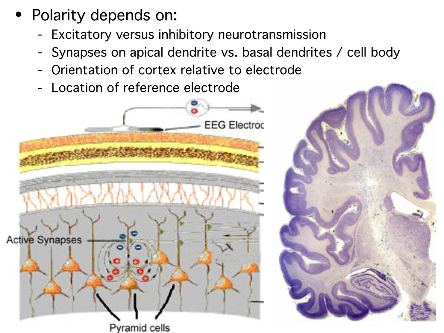
First, every ERP component will be positive on one side of the head and negative on the other side.  We often don't "see" the other side of a component (e.g., the negative side of the P3) because (a) the opposite-polarity side is in a place without any electrodes (e.g., the bottom of the skull), (b) the opposite-polarity side is obscured by other components, or (c) the opposite-polarity side is spatially diffuse (low amplitude and broadly distributed).  But it's there!

As the figure below shows, there are 4 factors that determine the polarity of an ERP component.  If we knew 3, we could in principle determine the 4th by knowing the polarity.  In practice, we never know 3 so we cannot determine the 4th.  In particular, although the polarity depends on whether the ERP arises from excitatory or inhibitory neurotransmission, we cannot ordinarily determine whether a component represents excitation or inhibition from its polarity.

Polarity.jpg

Mainly, polarity is used to help identify a given component.  For example, if our active electrodes are near Pz and our reference electrodes are near the mastoids, we can be sure that the P3 will be a positive voltage.  Beyond that, polarity doesn't tell us much.