Webinar on Standardized Measurement Error (a universal measure of ERP data quality)

We will be holding a webinar on our new universal measure of ERP data quality, which call the Standardized Measurement Error (SME). Check out this previous blog post for an overview of the SME and how you can use it.

The webinar will be presented by Steve Luck, and it will be held on Wednesday, August 5 at 8:00 AM Pacific Daylight Time (GMT-7). We expect that it will last 60-90 minutes. The timing is designed to allow the largest number of people to attend (even though it will be pretty early in the morning here in California!).

We will cover the basic logic behind the SME, how it can be used by ERP researchers, and how to calculate it for your own data using ERPLAB Toolbox (v8 and higher).

If you can’t attend, we will make a recording available for 1 week after the webinar. The link to the recording will be provided on the Virtual ERP Boot Camp page within 24 hours of the end of the webinar.

Advance registration is required and will be limited to the first 950 registrants. You can register at https://ucdavis.zoom.us/webinar/register/WN_LYlHHglWT2mkegGQdtr-Gg. You do NOT need to register to watch the recording.

When you register, you will immediately receive an email with an individualized Zoom link. If you do not see the email, check your spam folder. If you still don’t see it, you may have entered your email address incorrectly.

Questions can be directed to erpbootcamp@gmail.com.

Announcing the Release of ERP CORE: An Open Resource for Human Event-Related Potential Research

We are excited to announce the official release of the ERP CORE, a freely available online resource we developed for the ERP community. The ERP CORE was designed to help everyone from novice to experienced ERP researchers advance their program of research in several distinct ways.

The ERP CORE includes: 1) experiment control scripts for 6 optimized ERP paradigms that collectively elicit 7 ERP components (N170, MMN, N2pc, N400, P3, LRP, and ERN) in just one hour of recording time, 2) raw and processed data from 40 neurotypical young adults in each paradigm, 3) EEG/ERP data processing pipelines and analysis scripts in EEGLAB and ERPLAB Matlab Toolboxes, and 4) a broad set of ERP results and EEG/ERP data quality measures for comparison across laboratories.

A paper describing the ERP CORE is available here, and the online resource files are accessible here. Below we detail just some of the ways in which ERP CORE may be useful to ERP researchers.

• The ERP CORE provides a comprehensive introduction to the analysis of ERP data, including all processing steps, parameters, and the order of operations used in ERP data analysis. As a result, this resource can be used by novice ERP researchers to learn how to analyze ERP data, or by researchers of all levels who wish to learn ERP data analysis using the open source EEGLAB and ERPLAB Matlab Toolboxes. More advanced researchers can use the annotated Matlab scripts as a starting point for scripting their own analyses. Our analysis parameters, such as time windows and electrode sites for measurement, could also be used as a priori parameters in future studies, reducing researcher degrees of freedom.

• With data for 7 ERP components in 40 neurotypical research participants, the provided ERP CORE data set could be reanalyzed by other researchers to test new hypotheses or analytic techniques, or to compare the effectiveness of different data processing procedures across multiple ERP components. This may be particularly useful to researchers right now, given the limitations many of us are facing in collecting new data sets.

• The experiment control scripts for each of the ERP CORE paradigms we designed are provided in Presentation software for use by other researchers. Each paradigm was specifically designed to robustly elicit a specific ERP component in a brief (~10 min) recording. The experiment control scripts were programmed to make it incredibly easy for other researchers to directly use the tasks in their laboratories. For example, the stimuli can be automatically scaled to the same sizes as in our original recording by simply inputting the height, width, and viewing distance of the monitor you wish to use to collect data in your lab. The experiment control scripts are also easy to modify using the parameters feature in Presentation, which allows changes to be made to many features of the task (e.g., number of trials, stimulus duration) without modifying the code. Thus, the ERP CORE paradigms could be added on to an existing study, or be used as a starting point for the development of new paradigms.

• We provide several metrics quantifying the noise levels of our EEG/ERP data that may be useful as a comparison for both novice and experienced ERP researchers to evaluate their laboratory set-up and data collection procedures. The quality of EEG/ERP data plays a big role in statistical power; however, it can be difficult to determine the overall quality of ERP data in published papers. This makes it difficult for a given researcher to know whether their data quality is comparable to that of other labs. The ERP CORE provides measures of data quality for our data, as well as analysis scripts and procedures that other researchers can use to calculate these same data quality metrics on their own data.

These are just some of the many ways we anticipate that the ERP CORE will be used by ERP researchers. We are excited to see what other uses you may find for this resource and to hear feedback on the ERP CORE from the ERP community.

A New Metric for Quantifying ERP Data Quality

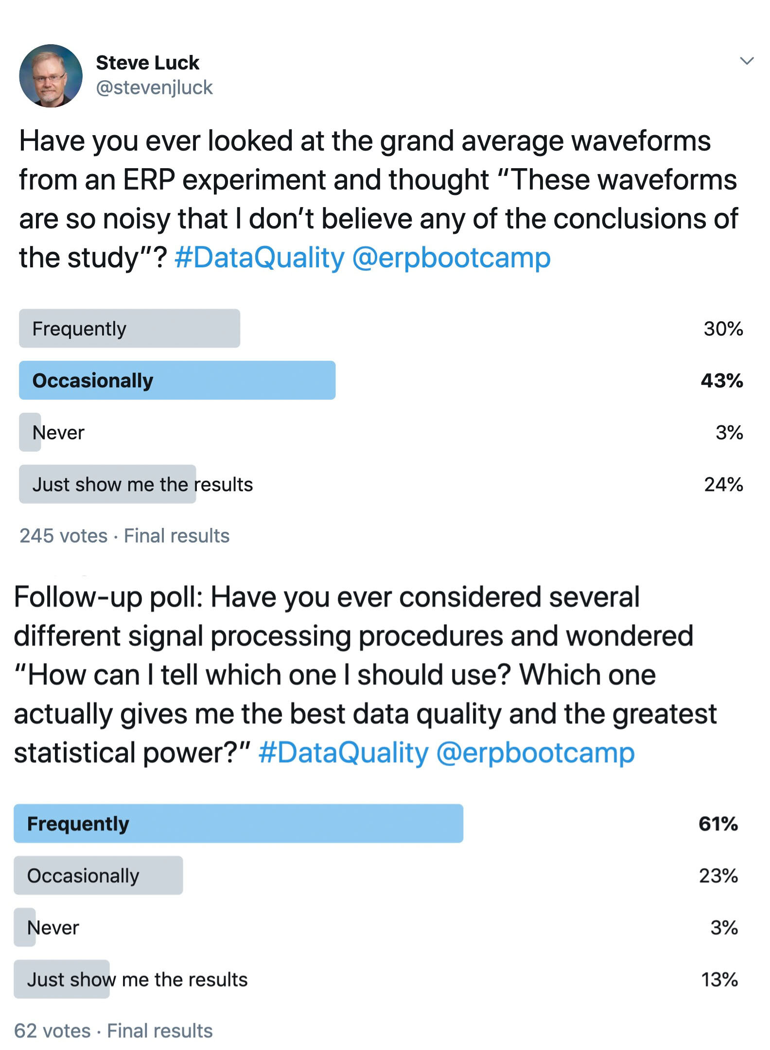
I’ve been doing ERP research for over 30 years, and for that entire time I have been looking for a metric of data quality. I’d like to be able to quantify the noise in my data in a variety of different paradigms, and I’d like to be able to determine exactly how a given signal processing operation (e.g., filtering) changes the signal-to-noise ratio of my data. And when I review a manuscript with really noisy-looking data, making me distrust the conclusions of the study, I’d like to be able to make an objective judgment rather than a subjective judgment. Given the results of the Twitter polls shown here, a lot of other people would also like to have a good metric of data quality.

I’ve looked around for such a metric for many years, but I never found one. So a few years ago, I decided that I should try to create one. I enlisted the aid of Andrew Stewart, Aaron Simmons, and Mijke Rhemtulla, and together we’ve developed a very simple but powerful and flexible metric of data quality that we call the Standardized Measurement Error or SME.

The SME has 3 key properties:

1. It reflects the extent to which noise (i.e., trial-to-trial variations in the EEG recording) impacts the score that you are actually using as the dependent variable in your study (e.g., the peak latency of the P3 wave). This is important, because the effect of noise will differ across different amplitude and latency measures. For example, high-frequency noise will have a big impact on the peak amplitude between 300 and 500 ms but relatively little impact on the mean voltage during this time range. The impact of noise depends on both the nature of the noise and what you are trying to measure.

2. It quantifies the data quality for each individual participant at each electrode site of interest, making it possible to determine (for example) whether a given participant’s data are so noisy that the participant should be excluded from the statistical analyses or whether a given electrode should be interpolated.

3. It can be aggregated across participants in a way that allows you to estimate the impact of the noise on your effect sizes and statistical power and to estimate how your effect sizes and power would change if you increased or decreased the number of trials per participant.

The SME is a very simple metric: It’s just the standard error of measurement of the score of interest (e.g., the standard error of measurement for the peak latency value between 300 and 500 ms). It is designed to answer the question: If I repeated this experiment over and over again in the same participant (assuming no learning, fatigue, etc.), and I obtained the score of interest in each repetition, how similar would the scores be across repetitions? For example, if you repeated an experiment 10,000 times in a given participant, and you measured P3 peak latency for each of the 10,000 repetitions, you could quantify the consistency of the P3 peak latency scores by computing the standard deviation (SD) of the 10,000 scores. The SME metric provides a way of estimating this SD using the data you obtained in a single experiment with this participant.

The SME can be estimated for any ERP amplitude or latency score that is obtained from an averaged ERP waveform. If you quantify amplitude as the mean voltage across some time window (e.g., 300-500 ms for the P3 wave), the SME is trivial to estimate. If you want to quantify peak amplitude or peak latency, you can still use the SME, but it requires a somewhat more complicated estimation technique called bootstrapping. Bootstrapping is incredibly flexible, and it allows you to estimate the SME for very complex scores, such as the onset latency of the N2pc component in a contralateral-minus-ipsilateral difference wave.

Should you start using the SME to quantify data quality in your own research? Yes!!! Here are some things you could do if you had SME values:

• Determine whether your data quality has increased or decreased when you modify a data analysis step or experimental design feature

• Notice technical problems that are reducing your data quality (e.g., degraded electrodes, a poorly trained research assistant) 

• Determine whether a given participant’s data are too noisy to be included in the analyses or whether a channel is so noisy that it should be replaced with interpolated values

• Compare different EEG recording systems, different recording procedures, and different analysis pipelines to see which one yields the best data quality

The SME would be even more valuable if researchers started regularly including SME values in their publications. This would allow readers/reviewers to objectively assess whether the results are beautifully clean, unacceptably noisy, or somewhere in between. Also, if every ERP paper reported the SME, we could easily compare data quality across studies, and the field could determine which recording and analysis procedures produce the cleanest data. This would ultimately increase the number of true, replicable findings and decrease the number of false, unreplicable findings. 

My dream is that, 10 years from now, every new ERP manuscript I review and every new ERP paper I read will contain SME values (or perhaps some newer, better measure of data quality that someone else will be inspired to develop).

To help make that dream come true, we’re doing everything we can to make it easy for people to compute SME values. We’ve just released a new version of ERPLAB Toolbox (v8.0) that will automatically compute the SME using default time windows every time you make an averaged ERP waveform. These SME values will be most appropriate when you are scoring the amplitude of an ERP component as the mean voltage during some time window (e.g., 300-500 ms for the P3 wave), but they also give you an overall sense of your data quality.  If you are using some other method to score your amplitudes or latencies (e.g., peak latency), you will need to write a simple Matlab script that uses bootstrapping to estimate the SME. However, we have provided several example scripts, and anyone who knows at least a little bit about Matlab scripting should be able to adapt our scripts for their own data. And we hope to add an automated method for bootstrapping in future versions of ERPLAB.

By now, I’m sure you’ve decided you want to give it a try, and you’re wondering where you can get more information.  Here are links to some useful resources:

• Full-length paper about the SME

  • Luck, S. J., Stewart, A. X., Simmons, A. M., & Rhemtulla, M. (2021). Standardized measurement error: A universal metric of data quality for averaged event-related potentials. Psychophysiology, 58, e13793. https://doi.org/10.1111/psyp.13793 [Access free on National Library of Medicine]

• Preprint of a short overview of the SME

• ERPLAB Toolbox download page

• Overview of data quality measures in the ERPLAB Wiki

• Example data and scripts on OSF

• Paper using the SME to quantify data quality for 7 different ERP components (P3b, MMN, N400, N170, N2pc, LRP, ERN)

Step-by-Step Protocols for Collecting Clean EEG Data

Standard Version: Farrens, J. L., Simmons, A. M., Luck, S. J., & Kappenman, E. S. (2019). Electroencephalogram (EEG) Recording Protocol for Cognitive and Affective Human Neuroscience Research. Protocol Exchange. https://doi.org/10.21203/rs.2.18328/v2 [PDF]

COVID-19 Version: Simmons, A. M., & Luck, S. J. (2020). Protocol for Reducing COVID-19 Transmission Risk in EEG Research. Protocol Exchange. https://doi.org/10.21203/rs.3.pex-974/v2

We have published an in-depth description of our EEG recording procedures, which provides an extremely detailed, step-by-step account of how we currently record EEG data in our laboratories (along with a modified version to minimize risk of COVID-19 transmission). Although this level of detail important for collecting clean data, it would be unrealistic to include 20+ pages of recording details in the Method section of a journal article. By publishing this protocol and then citing it in our papers, other researchers will know exactly how we recorded our data, which will enhance reproducibility. In addition, this protocol provides a forum for sharing the tips and tricks we have developed for collecting clean EEG data, which may help you improve your data quality. We encourage other researchers to either follow and cite our protocol or publish and cite their own protocols. If you’d like more information about why we think this is important, read on…

If you’ve ever recorded or processed raw EEG data, you know how noisy the data can be. The neural signals we want to record are contaminated by a variety of biological and non-biological noise sources, including muscle activity (EMG), heartbeats (EKG), skin potentials, movement artifacts, and induced electrical noise from the environment. To maximize the likelihood of finding the neural effects of interest, researchers need to do everything they can to reduce the noise during a recording session. Postprocessing techniques such as filters can help, but they can’t eliminate all the noise, and they often have a cost (e.g., temporal distortion). This is why one of our ERP Boot Camp mottos is “There is no substitute for clean data!”

When you run an EEG recording session, there are a million little details that together impact the quality of the data. Every lab has its own approach, but our field has no widely used mechanism for sharing these methodological details. Recording methods are usually described in journal articles with only a brief mention of the recording parameters (e.g., filter settings and sampling rate) and no information about the millions of other details that impact data quality. And really, who would want to slog through a Method section that described how the electrodes were oriented in their holders or listed the specific make and model of chair that was used to ensure that the participant remained comfortable?

However, these details really matter. For example, we have shown that the temperature of the recording environment can have a substantial impact on statistical power (Kappenman & Luck, 2010), but we have never seen an EEG/ERP paper from another lab that mentioned the temperature of the recording room.

A mechanism now exists for reporting all of these details. Specifically, one can now easily publish a formal protocol that is permanent and citable (and even contributes to citation counts on Google Scholar, if you care about that sort of thing). There are a variety of ways to publish a protocol, but we chose Nature’s Protocol Exchange web site. It’s free, appears to be robust, and automatically generates a DOI. It does not involve peer review (because you are merely listing your procedures, not drawing any formal conclusions), but it does involve a quick administrative review (to make sure that inappropriate materials are not posted). The protocol is published with a Creative Commons license, so Nature does not own it, and anyone can use it. Other sites may be even better, but Protocol Exchange fits our current needs reasonably well (although we would have appreciated a little more control over the formatting).

We encourage other researchers to read our protocol and use it to get ideas for their own recording methods. Our methods may not be ideal for some kinds of research, and other labs may have equivalent or even better methods.

More than anything, we hope that our protocol inspires other researchers to start publishing their own detailed protocols. This sharing of information will help everyone collect the cleanest possible data, improving the quality of published research in our field. Detailed protocols will also increase reproducibility of research methods and perhaps even replicability of research findings. Note that our protocol is longer and more detailed that what most labs would publish (because we included advice about things like fixing broken electrodes).

You can find the standard version of the protocol at protocolexchange.researchsquare.com/article/663a5a19-c74e-4c7d-b3fc-9c5188332b46/v2 or at doi.org/10.21203/rs.2.18328/v2. You can download a nicely formatted PDF of the protocol here.

You can find the COVID-19 version at https://protocolexchange.researchsquare.com/article/pex-974/v2 or at https://doi.org/10.21203/rs.3.pex-974/v2

Why experimentalists should ignore reliability and focus on precision

It is commonly said that “a measure cannot be valid if it is not reliable.” It turns out that this is not true as these terms are typically defined in psychology. And it also turns out that, although reliability is extremely important in some types of research (e.g., correlational studies of individual differences), it’s the wrong way for most experimentalists to think about the quality of their measures.

I’ve been thinking about this issue for the last 2 years, as my lab has been working on a new method for quantifying data quality in ERP experiments (stay tuned for a preprint). It turns out that ordinary measures of reliability are quite unsatisfactory for assessing whether ERP data are noisy. This is also true for reaction time (RT) data. A couple days ago, Michaela DeBolt (@MDeBoltC) alerted me to a new paper by Hedge et al. (2018) showing that typical measures of reliability can be low even when power is high in experimental studies. There’s also a recent paper on MRI data quality by Brandmaier et al. (2018) that includes a great discussion of how the term “reliability” is used to mean different things in different fields.

Here’s a quick summary of the main issue: Psychologists usually quantify reliability using correlation-based measures such as Cronbach’s alpha. Because the magnitude of a correlation depends on the amount of true variability among participants, these measures of reliability can go up or down a lot depending on how homogeneous the population is. All else being equal, a correlation will be lower if the participants are more homogeneous. Thus, reliability (as typically quantified by psychologists) depends on the range of values in the population being tested as well as the nature of the measure. That’s like a physicist saying that the reliability of a thermometer depends on whether it is being used in Chicago (where summers are hot and winters are cold) or in San Diego (where the temperature hovers around 72°F all year long).

One might argue that this is not really what psychometricians mean when they’re talking about reliability (see Li, 2003, who effectively redefines the term “reliability” to capture what I will be calling “precision”). However, the way I will use the term “reliability” captures the way this term has been operationalized in 100% of the papers I have read that have quantified reliability (and in the classic texts on psychometrics cited by Li, 2003).

A Simple Reaction Time Example

Let’s look at this in the context of a simple reaction time experiment. Imagine that two researchers, Dr. Careful and Dr. Sloppy, use exactly the same task to measure mean RT (averaged over 50 trials) from each person in a sample of 100 participants (drawn from the same population). However, Dr. Careful is meticulous about reducing sources of extraneous variability, and every participant is tested by an experienced research assistant at the same time of day (after a good night’s sleep) and at the same time since their last meal. In contrast, Dr. Sloppy doesn’t worry about these sources of variance, and the participants are tested by different research assistants at different times of day, with no effort to control sleepiness or hunger. The measures should be more reliable for Dr. Careful than for Dr. Sloppy, right? Wrong! Reliability (as typically measured by psychologists) will actuallybe higher for Dr. Sloppy than for Dr. Careful (assuming that Dr. Sloppy hasn’t also increased the trial-to-trial variability of RT).

To understand why this is true, let’s take a look at how reliability would typically be quantified in a study like this. One common way to quantify the reliability of the RT measure is the split-half reliability. (There are better measures of reliability, but they all lead to the same problem, and split-half reliability is easy to explain.) To compute the split-half reliability, the researchers divide the trials for each participant into odd-numbered and even-numbered trials, and they calculate the mean RT separately for the odd- and even-numbered trials. This gives them two values for each participant, and they simply compute the correlation between these two values. The logic is that, if the measure is reliable, then the mean RT for the odd-numbered trials should be pretty similar to the mean RT for the even-numbered trials in a given participant, so individuals with a fast mean RT for the odd-numbered trials should also have a fast mean RT for the even-numbered trials, leading to a high correlation. If the measure is unreliable, however, the mean RTs for the odd- and even-numbered trials will often be quite different for a given participant, leading to a low correlation.

However, correlations are also impacted by the range of scores, and the correlation between the mean RT for the odd- versus even-numbered trials will end up being greater for Dr. Sloppy than for Dr. Careful because the range of mean RTs is greater for Dr. Sloppy (e.g., because some of Dr. Sloppy’s participants are sleepy and others are not). This is illustrated in the scatterplots below, which show simulations of the two experiments. The experiments are identical in terms of the precision of the mean RT measure (i.e., the trial-to-trial variability in RT for a given participant). The only thing that differs between the two simulations is the range of true mean RTs (i.e., the mean RT that a given participant would have if there were no trial-by-trial variation in RT). Because all of Dr. Careful’s participants have mean RTs that cluster closely around 500 ms, the correlation between the mean RTs for the odd- and even-numbered trials is not very high (r=.587). By contrast, because some of Dr. Sloppy’s participants are fast and others are slow, the correlation is quite good (r=.969). Thus, simply by allowing the testing conditions to vary more across participants, Dr. Sloppy can report a higher level of reliability than Dr. Careful. 

Keep in mind that Dr. Careful and Dr. Sloppy are measuring mean RT in exactly the same way. The actual measure is identical in their studies, and yet the measured reliability differs dramatically across the studies because of the differences in the range of scores. Worse yet, the sloppy researcher ends up being able to report higher reliability than the careful researcher.

Let’s consider an even more extreme example, in which the population is so homogeneous that every participant would have the same mean RT if we averaged together enough trials, and any differences across participants in observed mean RT are entirely a result of random variation in single-trial RTs. In this situation, the split-half reliability would have an expected value of zero. Does this mean that mean RT is no longer a valid measure of processing speed? Of course not—our measure of processing speed is exactly the same in this extreme case as in the studies of Dr. Careful and Dr. Sloppy. Thus, a measure can be valid even if it is completely unreliable (as typically quantified by psychologists).

Here’s another instructive example. Imagine that Dr. Careful does two studies, one with a population of college students at an elite university (who are relatively homogeneous in age, education, SES, etc.) and one with a nationally representative population of U.S. adults (who vary considerably in age, education, SES, etc.). The range of mean RT values will be much greater in the nationally representative population than in the college student population. Consequently, even if Dr. Careful runs the study in exactly the same way in both populations, the reliability will likely be much greater in the nationally representative population than in the college student population. Thus, reliability (as typically measured by psychologists) depends on the range of scores in the population being measured and not just on the properties of the measure itself. This is like saying that a thermometer is more reliable in Chicago than in San Diego simply because the range of temperatures is greater in Chicago.

Example of an Experimental Manipulation

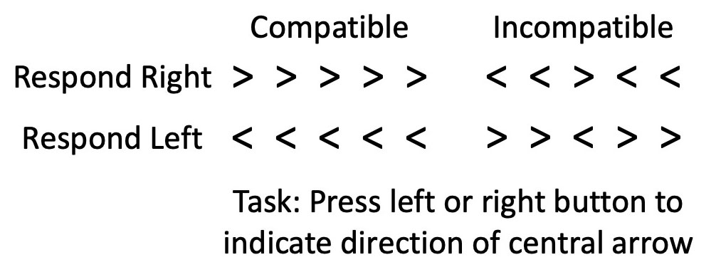
Now let’s imagine that Dr. Careful and Dr. Sloppy don’t just measure mean RT in a single condition, but they instead test the effects of a within-subjects experimental manipulation. Let’s make this concrete by imagining that they conduct a flankers experiment, in which participants report whether a central arrow points left or right while ignoring flanking stimuli that are either compatible or incompatible with the central stimulus (see figure to the right). In a typical study, mean RT would be slowed on the incompatible trials relative to the compatible trials (a compatibility effect).

If we look at the mean RTs in a given condition of this experiment, we will see that the mean RT varies from participant to participant much more in Dr. Sloppy’s version of the experiment than in Dr. Careful’s version (because there is more variation in factors like sleepiness in Dr. Sloppy’s version). Thus, as in our original example, the split-half reliability of the mean RT for a given condition will again be higher for Dr. Sloppy than for Dr. Careful. But what about the split-half reliability of the flanker compatibility effect? We can quantify the compatibility effect as the difference in mean RT between the compatible and incompatible trials for a given participant, averaged across left-response and right-response trials. (Yes, there are better ways to analyze these data, but they all lead to the same conclusions about reliability.) We can compute the split-half reliability of the compatibility effect by computing it twice for every subject—once for the odd-numbered trials and once for the even-numbered trials—and calculating the correlation between these values.

The compatibility effect, like the raw RT, is likely to vary according to factors like the time of day, so the range of compatibility effects will be greater for Dr. Sloppy than for Dr. Careful. And this means that the split-half reliability will again be greater for Dr. Sloppy than for Dr. Careful. (Here I am assuming that trial-to-trial variability in RT is not impacted by the compatibility manipulation and by the time of day, which might not be true, but nonetheless it is likely that the reliability will be at least as high for Dr. Sloppy as for Dr. Careful.)

By contrast, statistical power for determining whether a compatibility effect is present will be greater for Dr. Careful than for Dr. Sloppy. In other words, if we use a one-sample t test to compare the mean compatibility effect against zero, the greater variability of this effect in Dr. Sloppy’s experiment will reduce the power to determine whether a compatibility effect is present. So, even though reliability is greater for Dr. Sloppy than for Dr. Careful, statistical power for detecting an experimental effect is greater for Dr. Careful than for Dr. Sloppy. If you care about statistical power for experimental effects, reliability is probably not the best way for you to quantify data quality.

An Example of Individual Differences

What if Dr. Careful and Dr. Sloppy wanted to look at individual differences? For example, imagine that they were testing the hypothesis that the flanker compatibility effect is related to working memory capacity. Let’s assume that they measure both variables in a single session. Assuming that both working memory capacity and the compatibility effect vary as a function of factors like time of day, Dr. Sloppy will find greater reliability for both working memory capacity and the compatibility effect (because the range of values is greater for both variables in Dr. Sloppy’s study than in Dr. Careful’s study). Moreover, the correlation between working memory capacity and the compatibility effect will be higher in Dr. Sloppy’s study than in Dr. Careful’s study (again because of differences in the range of scores).

In this case, greater reliability is associated with stronger correlations, just as the psychometricians have always told us. All else being equal, the researcher who has greater reliability for the individual measures (Dr. Sloppy in this example) will find a greater correlation between them. So, if you want to look at correlations between measures, you want to maximize the range of scores (which will in turn maximize your reliability). However, recall that Dr. Careful had more statistical power than Dr. Sloppy for detecting the compatibility effect. Thus, the same factors that increase reliability and correlations between measures can end up reducing statistical power when you are examining experimental effects with exactly the same measures. (Also, if you want to look at correlations between RT and other measures, I recommend that you read Miller & Ulrich, 2013, which shows that these correlations are more difficult to interpret than you might think.)

It’s also important to note that Dr. Sloppy would run into trouble if we looked at test-retest reliability instead of split-half reliability. That is, imagine that Dr. Sloppy and Dr. Careful run studies in which each participant is tested on two different days. Dr. Careful makes sure that all of the testing conditions (e.g., time of day) are the same for every participant, but Dr. Sloppy isn’t careful to keep the testing conditions constant between the two session for each participant. The test-retest reliability (the correlation between the measure on Day 1 and Day 2) would be low for Dr. Sloppy. Interestingly, Dr. Sloppy would have high split-half reliability (because of the broad range of scores) but poor test-retest reliability. Dr. Sloppy would also have trouble if the compatibility effect and working memory capacity were measured on different days.

Precision vs. Reliability

Now let’s turn to the distinction between reliability and precision. The first part of the Brandmaier et al. (2018) paper has an excellent discussion of how the term “reliability” is used differently across fields. In general, everyone agrees that a measure is reliable to the extent that you get the same thing every time you measure it. The difference across fields lies in how reliability is quantified. When we think about reliability in this way, a simple way to quantify it would be to obtain the measure a large number of times under identical conditions and compute the standard deviation (SD) of the measurements. The SD is a completely straightforward measure of the “the extent that you get the same thing every time you measure it.” For example, you could use a balance to weigh an object 100 times, and the standard deviation of the weights would indicate the reliability of the balance. Another term for this would be the “precision” of the balance, and I will use the term “precision” to refer to the SD over multiple measurements. (In physics, the SD is typically divided by the mean to get the coefficient of variability, which is often a better way to quantify reliability for measures like weight that are on a ratio scale.)

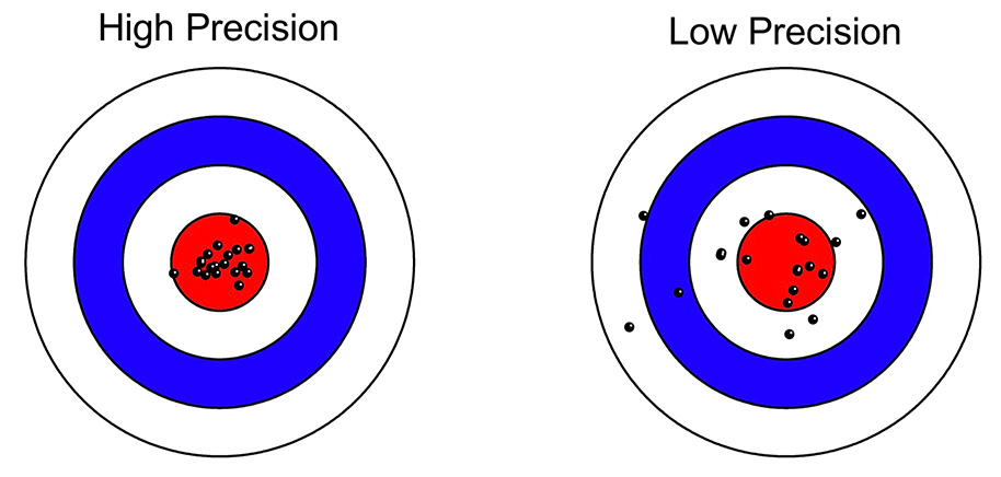
The figure below (from the Brandmaier article) shows what is meant by low and high precision in this context, and you can see how the SD would be a good measure of precision. The key is that precision reflects the variability of the measure around its mean, not whether the mean is the true mean (which would be the accuracy or bias of the measure).

Things are more complicated in most psychology experiments, where there are (at least) two distinct sources of variability in a given experiment: true differences among participants (called the true score variance) and measurement imprecision. However, in a typical experiment, it is not obvious how to separately quantify the true score variance from the measurement imprecision. For example, if you measure a dependent variable once from N participants, and you look at the variance of those values, the result will be the sum of the true score variance and the variance due to measurement error. These two sources of variance are mixed together, and you don’t know how much of the variance is a result of measurement imprecision.

Imagine, however, that you’ve measured the dependent variable twice from each subject. Now you could ask how close the two measures are to each other. For example, if we take our original simple RT experiment, we could get the mean RT from the odd-number trials and the mean RT from the even-numbered trials in each participant. If these two scores were very close to each other in each participant, then we would say we have a precise measure of mean RT. For example, if we collected 2000 trials from each participant, resulting in 1000 odd-numbered trials and 1000 even-numbered trials, we’d probably find that the two mean RTs for a given subject were almost always within 10 ms of each other. However, if collected only 20 trials from each participant, we would see big differences between the mean RTs from the odd- and even-numbered trials. This makes sense: All else being equal, mean RT should be a more precise measure if it’s based on more trials.

In a general sense, we’d like to say that mean RT is a more reliable measure when it’s based on more trials. However, as the first part of this blog post demonstrated, typical psychometric approaches to quantifying reliability are also impacted by the range of values in the population and not just the precision of the measure itself: Dr. Sloppy and Dr. Careful were measuring mean RT with equal precision, but split-half reliability was greater for Dr. Careful than for Dr. Sloppy because there was a greater range of mean RT values in Dr. Sloppy’s study. This is because split-half reliability does not look directly at how similar the mean RTs are for the odd- and even-numbered trials; instead, it involves computing the correlation between these values, which in turn depends on the range of values across participants.

How, then, can we formally quantify precision in a way that does not depend on the range of values across participants? If we simply took the difference in mean RT between the odd- and even-numbered trials, this score would be positive for some participants and negative for others. As a result, we can’t just average this difference across participants. We could take the absolute value of the difference for each participant and then average across participants, but absolute values are problematic in other ways. Instead, we could just take the standard deviation (SD) of the two scores for each person. For example, if Participant #1 had a mean RT of 515 ms for the odd-numbered trials and a mean RT of 525 ms for the even-numbered trials, the SD for this participant would be 7.07 ms. SD values are always positive, so we could average the single-participant SD values across participants, and this would give us an aggregate measure of the precision of our RT measure.

The average of the single-participant SDs would be a pretty good measure of precision, but it would underestimate the actual precision of our mean RT measure. Ultimately, we’re interested in the precision of the mean RT for all of the trials, not the mean RT separately for the odd- and even-numbered trials. By cutting the number of trials in half to get separate mean RTs for the odd- and even-numbered trials, we get an artificially low estimate of precision.

Fortunately, there is a very familiar statistic that allows you to quantify the precision of the mean RT using all of the trials instead of dividing them into two halves. Specifically, you can simply take all of the single-trial RTs for a given participant in a given condition and compute the standard error of the mean (SEM). This SEM tells you what you would expect to find if you computed the mean RT for that subject in each of an infinite number of sessions and then took the SD of the mean RT values.

Let’s unpack that. Imagine that you brought a single participant to the lab 1000 times, and each time you ran 50 trials and took the mean RT of those 50 trials. (We’re imagining that the subject’s performance doesn’t change over repeated sessions; that’s not realistic, of course, but this is a thought experiment so it’s OK.) Now you have 1000 mean RTs (each based on the average of 50 trials). You could take the SD of those 1000 mean RTs, and that would be an accurate way of quantifying the precision of the mean RT measure. It would be just like a chemist who weighs a given object 1000 times on a balance and then uses the SD of these 1000 measurements to quantify the precision of the balance.

But you don’t actually need to bring the participant to the lab 1000 times to estimate the SD. If you compute the SEM of the 50 single-trial RTs in one session, this is actually an estimate of what would happen if you measured mean RT in an infinite number of sessions and then computed the SD of the mean RTs. In other words, the SEM of the single-trial RTs in one session is an estimate of the SD of the mean RT across an infinite number of sessions. (Technical note: It would be necessary to deal with the autocorrelation of RT across trials, but there are methods for that.)

Thus, you can use the SEM of the single-trial RTs in a given session as a measure of the precision of the mean RT measure for that session. This gives you a measure of the precision for each individual participant, and you can then just average these values across participants. Unlike traditional measures of reliability, this measure of precision is completely independent of the range of values across the population. If Dr. Careful and Dr. Sloppy used this measure of precision, they would get exactly the same value (because they’re using exactly the same procedure to measure mean RT in a given participant). Moreover, this measure of precision is directly related to the statistical power for detecting differences between conditions (although there is a trick for aggregating the SEM values across participants, as will be detailed in our paper on ERP data quality).

So, if you want to assess the quality of your data in an experimental study, you should compute the SEM of the single-trial values for each subject, not some traditional measure of “reliability.” Reliability is very important for correlational studies, but it’s not the right measure of data quality in experimental studies.

Here’s the bottom line: the idea that “a measure cannot be valid if it is not reliable” is not true for experimentalists (given how reliability is typically operationalized by psychologists), and they should focus on precision rather than reliability.

How Many Trials Should You Include in Your ERP Experiment?

Boudewyn, M. A., Luck, S. J., Farrens, J. L., & Kappenman, E. S. (in press). How many trials does it take to get a significant ERP effect? It depends. Psychophysiology.

One question we often get asked at ERP Boot Camps is how many trials should be included in an experiment to obtain a stable and reliable version of a given ERP component. It turns out there is no single answer to this question that can be applied across all ERP studies. 

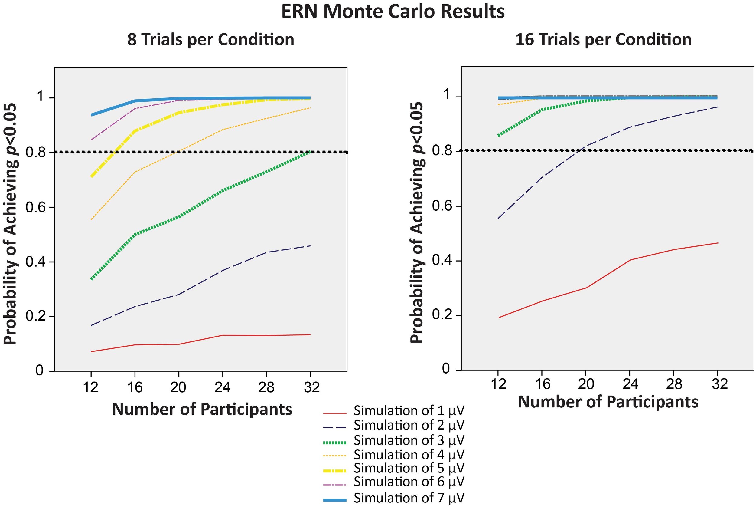
In a recent paper published in Psychophysiology in collaboration with Megan Boudewyn, a project scientist at UC Davis, we demonstrated how the number of trials, the number of participants, and the magnitude of the effect interact to influence statistical power (i.e., the probability of obtaining p<.05). One key finding was that doubling the number of trials recommended by previous studies led to more than a doubling of statistical power under many conditions. Interestingly, increasing the number of trials had a bigger effect on statistical power for within-participants comparisons than for between-group analyses. 

The results of this study show that a number of factors need to be considered in determining the number of trials needed in a given ERP experiment, and that there is no magic number of trials that can yield high statistical power across studies. 

Replication, Robustness, and Reproducibility in Psychophysiology

Interested in learning more about issues affecting reproducibility and replication in psychophysiological studies? Check out the articles in this special issue of Psychophysiology edited by Andreas Keil and me featuring articles by many notable researchers in the field.

Andreas and I will be discussing these issues and more with other researchers at a panel the opening night of the Society for Psychophysiological Research (SPR) annual meeting in Quebec City October 3-7. 

How to p-hack (and avoid p-hacking) in ERP Research

Luck, S. J., & Gaspelin, N. (2017). How to Get Statistically Significant Effects in Any ERP Experiment (and Why You Shouldn’t). Psychophysiology, 54, 146-157.

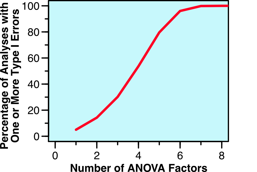
In this article, we show how ridiculously easy it is to find significant effects in ERP experiments by using the observed data to guide the selection of time windows and electrode sites. We also show that including multiple factors in your ANOVAs can dramatically increase the rate of false positives (Type I errors). We provide some suggestions for methods to avoid inflating the Type I error rate.

This paper was part of a special issue of Psychophysiology on Reproducibility edited by Emily Kappenman and Andreas Keil.